Prediction analysis of cotton yield based on BP neural network and multiple linear regression

1. Introduction

With the development of the economy and production level, the output of agricultural products has gradually increased. Therefore, it is particularly important to analyze the factors that affect the output of agricultural products. Cotton is selected as a representative agricultural product in this research to investigate the factors affecting its yield. By intercepting the official data on cotton production this year, multiple indicators are defined (fertilizer cost, consumption of agricultural plastic, pesticide cost,seed cost, irrigation cost, chlorpyrifos control area, labor input), and the relationship between cotton production and various indicators is analyzed using the Back Propagation (BP) neural network and multiple linear regression methods.

The relationship between cotton yield and various indicators is analyzed using the method of BP neural network and multiple linear regression, and the two methods are compare to find the method with less prediction error. Meanwhile, it analyzes the relationship between each factor and the unit yield, and gives suggestions on how to improve the cotton unit yield.

Through the forecasting cotton production and analyzing the related factors affecting production, future cotton production can be predicted more accurately, and the proportion of various factors affecting cotton production can be adjusted at present stage according to the forecasted results in order to increase cotton production. It is also to optimize the production input at the current stage, to achieve a larger unit output.

2. Methodology

2.1. The experiment data

Through searching and sorting in the National Bureau of Statistics, the Ministry of Agriculture, and the China Cotton Network, new information and relevant data have been obtained. The data is selected according to the year as the selection criterion,and the data is preprocessed in order to get a uniform unit. Due to the large amount of data, only part of it is shown in Table 1.

Table 1. Experiment data (Some data omitted)

2.2. Research methods

2.2.1. Determine the input and output objects By consulting relevant information and literature, seven factors were selected as independent variables that may affect the unit cotton yield, including: fertilizer cost, consumption of agricultural plastic film, pesticide cost, seed cost, irrigation cost, chlorpyrifos control area, and labor input [1-2]. Therefore, with these seven factors as input variables, cotton yield per unit is the dependent variable.

2.2.2. Data preprocessing Before neural network training, in order to avoid overfitting, 70% of the experimental data is used as the training set, 15% as the test set, and 15% as the validation set. Meanwhile, in order to eliminate the dimension between the data, the data is normalize [3].

2.2.3. BP neural network model The collected data is first normalized, and use Matlab's Mapminmax function to normalize the original data to [0,1].Then, using the levenberg marquardt algorithm, 10 neurons are set in the hidden layer of the neural network for training, and setting the number of training times, learning rate, and recording training target minimum error[4].

2.2.4. Multiple linear regression model The least squares method is used for multiple linear regression analysis, with 7 factors as input variables, and the unit output as output variables, with a confidence interval of 0.05 (alpha = 0.05), multiple linear regression analysis was performed to obtain the objective function for unit output. Applying the indicators established in the model, the least squares method is used to derive the multiple regression coefficients, and then calculate the probit values needed to obtain a comprehensive evaluation of the rank sum ratio[4].

2.2.5. Model validation In order to test the effectiveness of the model and verify model performance, after the BP neural network model is established and the training samples are trained, make a scatter plot of its regression and calculate the R square. Meanwhile, prediction error (PE) is calculating. For the multiple linear regression model, Durbin Watson test, P inspection, F inspection, and residual normality test are used to verify the validity of the model .

2.3. Notations

The symbols are shown in the following : Y as unit output, X1 as fertilizer cost, X2 as consumption of agricultural plastic film, X3 as pesticide cost, X4 as seed cost, X5 as irrigation cost, X6 as chlorpyrifos control area, and X7 as labor input.

3. Experiment and result

3.1. BP neural network model result

3.1.1. Various network parameters of the BP neural network model Using the collected data to build a BP neural network model, 7 factors are input as dependent variables, cotton unit yield is used as output data, and a 3-layer BP neural network model is established. Through multiple debugging of the data, it is finally concluded that the maximum number of training times is 2500, the initial learning rate is set to 0.001, the final learning rate is 0.000000001( gradient descent algorithm), the minimum error of the training target is 0.00000000001, and the others are default values.

3.1.2. The prediction value of BP neural network model and the accuracy of the model According to the model results in Table 2, the model errors of the verification group are all less than 5%, the ratio of the error to less than 10% is 100%, the accuracy rate of the model exceeds 99%, the average percentage error is 0.37%, and the average prediction error is 0.4%. Therefore, it can be considered that the BP nerve is used for prediction. The accuracy is relatively high. Moreover, a strong correlation was found between actual output and predicted output (r = 0.9956).

Table 2. BP neural network model verification group prediction results

3.1.3. BP neural network Correlation (R square) Use the correlation function to obtain the correlation coefficient matrix between the predicted unit output and the actual unit output, and then only take out the data in the second row and the first column of the matrix as the correlation coefficient (R square) to judge the correlation between the predicted value and the actual value. According to figure 1, it can be concluded that the R square is 0.99474 (overall), indicating that the correlation between the predicted unit output and the actual unit output is high.

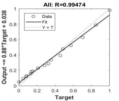
Figure 1. Correlation coefficient for predicting unit output

3.2. Multiple Linear Regression Model

3.2.1. Regression equation Input 7 factors as independent variables and output unit output as dependent variable to construct a multiple linear regression equation (confidence interval = 0.05). The multivariate linear equation is obtained (with regard to unit output):

3.2.2. Model statistical test According to Table 3, it is found that the R square is 0.991, indicating that the five indicators we have specified have an impact of 0.991 on the change of the dependent variable ( Means that these five indicators can explain 99.1% of the variation in the dependent variable). It can be considered that the 7 factors specified have played a greater role in the fluctuation of the dependent variable. It means that the predicted value is closer to the real value.

Table 3. Results of statistical tests

The value of Durbin Watson is 1.561, which is close to 2. Therefore, it can be seen that the 7 factors are independent of each other (samples are independent), and the predicted value is less affected by the endogeneity of the data. It can be seen that the result of this regression model can be seen effectively.

F inspection: if F>F1-alpha(m,n-m-1), it can be described as having a significant linear correlation between the dependent variable Y and the independent variables X1, X2, X3, X4, X5, X6, X7 (m=Number of independent variables, n=Statistical quantity,alpha = 0.05). In the model, by consulting the F distribution table, it can be concluded that the model has a significant liner correlation between the dependent variable Y and the independent variables X1, X2, X3, X4, X5, X6, X7.

In order to be sure that the model is effective, it is necessary to perform residual checkout. Therefore, graphs are plotted and check for normality. According to figure 2 (normalization residual normal P-P plot), it can be found that, points roughly fall on the straight line of y=x. Therefore, the residual data obeys normal distribution, and the residual analysis can be passed [5].

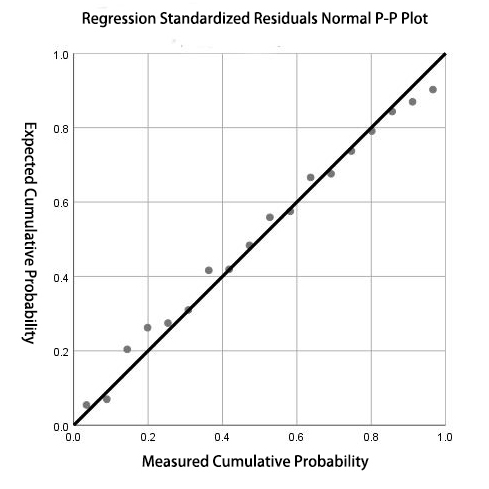
Figure 2. Regression normalization residual normal P-P plot

3.2.3. Multiple linear regression model error analysis The results of multiple linear regression model verification accounted for 90% of the test set with an error of less than 10%, and 7% of which had an error of less than 15%. Meanwhile, using corrcoef function to find the correlation coefficient between actual unit production and predicted unit production, a strong correlation was found between actual and predicted yields (r = 0.9520).

4. Discussion

The paper constructed two prediction models to predict unit cotton yield, BP neural network model and multiple linear regression model. To explore the various factors that affect the unit cotton yield. This search found that the input of chemical fertilizers and pesticides has a significant impact on the unit cotton yield, and it is significantly positively correlated. Moreover, consumption of agricultural plastic film and chlorpyrifos control areas has no significant effect on unit cotton yield. Therefore, it can be suggested to appropriately increase the input of chemical fertilizers and pesticides in the production of cotton[6].

In this experiment, by comparing the two models, it can be inferred that the prediction model of cotton unit yield has a strong linear correlation, and the prediction and fitting of the multiple linear regression model also have higher accuracy [7].

However, comparing the prediction accuracy of the two models of BP neural network and multiple linear regression, it can be found that the prediction accuracy of BP neural network is better, but the accuracy of multiple linear regression is relatively more accurate. The correlation coefficients between the actual unit output and the predicted unit output of the two are more than 0.95, among which the correlation coefficient of the BP neural network model is 0.9956, and the correlation coefficient of the multiple linear regression model is 0.9520. Therefore, although the BP neural network is a non-linear forecast, it is still possible to obtain more accurate unit output forecast data by adjusting the learning rate, maximum training times, and other parameters to support the training ability and self-learning ability of the BP neural network itself. It can be considered that both models have better accuracy in predicting the unit cotton yield, and the BP neural network is more accurate and can be used as a better method for prediction [8-10].

5. Conclusion

In this paper, BP neural network model and multiple linear regression model are used to predict. Through comparison, it is found that the accuracy of the BP neural network in predicting the unit cotton yield is higher than that of multiple linear regression. But the accuracy of the unit yield prediction using the two models is relatively high, and it can be roughly inferred that the factors affecting the cotton unit yield have a roughly linear relationship. This paper only uses two models of BP neural network and multiple linear regression in the discussion of unit cotton yield prediction, which has certain limitations. For this topic, LSTM deep learning, RNN neural network, and other models can also be used for analysis.