Research on tail risk measurement and risk spillover effects in financial markets

1. Introduction

At the 13th collective study session of the Political Bureau of the CPC Central Committee, General Secretary Xi Jinping emphasized that financial security is a critical component of national security. Scientifically identifying potential risk points within the operation of China's financial system is fundamental to constructing an effective financial security defense line. As a typical characteristic of systemic risk, financial market risk is inherently non-diversifiable. It not only transmits internally through risk spillovers among financial sub-markets [1] but also interacts bidirectionally with the macroeconomy via procyclical behaviors and financial accelerator mechanisms, thereby exacerbating the instability and fragility of the financial system [2]. Against the backdrop of downward pressure on the real economy and the accumulation of financial risks, exploring the dynamic evolution of financial market risks and examining their cross-market transmission mechanisms is essential for deepening the understanding of the relationship between macroeconomic trends and financial operations. Moreover, such exploration can provide empirical support and policy insights for improving risk prevention systems and formulating scientifically grounded macro-regulation and supervisory strategies.

Amid accelerating financial innovation and the dismantling of institutional barriers [3], the rapid iteration of cross-market financial products [4], the evolution of mixed-operation models [5], and the gradual relaxation of capital controls [6] are reshaping the operational logic of modern financial markets. The transmission and linkage of risks across multidimensional markets have intensified [7]. Risk exposures in specific domains [8] may trigger chain reactions in various sub-markets through channels such as liquidity spirals, asset-liability linkages [9], and behavioral expectation resonance [10], transforming price fluctuations in a single market into systemic pressure and ultimately exerting multiple negative impacts on the real economy [11]. In response, Holló et al. [12] innovatively proposed a multidimensional quantitative framework for measuring systemic financial risk using loss and uncertainty indicators across financial institutions, equity markets, bond markets, and foreign exchange markets. Subsequent studies have expanded upon this by incorporating other systemically relevant markets—such as the shadow banking sector [13], real estate market [14], and government sector [15]—to capture a more comprehensive profile of systemic risk.

It is noteworthy that as systemic risk accumulates, financial market risk intensifies and imposes significant negative externalities on the macroeconomy. Adrian and Brunnermeier [16] introduced the Conditional Value at Risk (CoVaR) model, which applies quantile regression to the measurement of systemic risk. By estimating financial institutions' risk exposures at extreme quantiles (e.g., the 95th percentile), the model quantifies their marginal contribution to systemic risk. Leveraging their ability to capture tail information in data distributions, quantile models have become ideal tools for depicting the asymmetric impacts of financial risks on macroeconomic conditions. Giglio [17] was the first to use partial quantile regression to characterize this asymmetry. In China, He Qing et al. [18] and Ouyang Zisheng et al. [19] applied this approach to construct systemic financial risk indices. Li Zheng et al. [20] and Yang Zihui et al. [21] employed LASSO quantile regression and multivariate conditional autoregressive quantile models, respectively, to build extreme risk networks and quantify tail risk spillovers. More recently, Yang Zihui et al. [22] adopted conditional quantile regression to investigate the heterogeneous impacts of various factors across quantiles, providing evidence for more precise control of imported risks.

With the advancement of scientific research and information technology, traditional methods are increasingly constrained in handling unstructured and high-dimensional data and capturing complex inter-variable relationships. New data-driven approaches such as machine learning are increasingly employed in the measurement and monitoring of financial risk. In line with the 3V characteristics of big data—volume, variety, and velocity—three focal areas have emerged: (1) Complex structure discovery: Fan Xiaoyun et al. [23] used text mining to capture the state of financial markets and assess systemic risk in China’s banking industry by analyzing co-occurring news sentiment related to banks; (2) Large-scale data processing: the inherent nonlinearity, heterogeneity, dynamism, and discreteness of big data provide the possibility, feasibility, and necessity for integrating machine learning into financial risk analysis [24]; (3) High-dimensional data analysis: due to the high-dimensional and time-varying nature of inter-market risk linkages in the financial system, traditional econometric models suffer from the “curse of dimensionality,” prompting scholars to adopt machine learning methods to address high-dimensional problems [25].

In summary, while existing literature on financial market risk has yielded fruitful results and provides valuable references for this study, there remain areas for further improvement: First, there is room for innovation in integrating high-dimensional features with analytical methods—specifically, how to retain the nonlinear properties of data while capturing the asymmetric effects of financial risks on the macroeconomy. Second, the systematic application of unstructured data is still lacking. The integration of unstructured data reflecting economic agents' risk perception and preferences with traditional financial indicators remains exploratory, limiting our ability to capture the nonlinear amplification effect of the “emotion accelerator” mechanism. Third, existing studies on quantile-based multidimensional linkages mainly focus on individual markets or institutions, and have yet to fully clarify the multi-dimensional interplay between financial sub-markets (e.g., financial institutions, stock, currency markets) and economic agents' risk perceptions.

In response, this paper constructs a research framework of “multidimensional indicator system → financial market risk characterization → financial risk contagion.” First, the RReliefF-RF-RFE method is used for feature selection, and a National Sentiment Index is developed to measure economic agents’ risk perceptions. The Quantile XGBoost+SHAP model is then employed to capture the risk factors through which financial markets impact the macroeconomy, thereby characterizing the asymmetric effects of financial risks. Second, the QVAR-DY model is applied to analyze the static spillover effects among financial sub-markets, economic agents’ risk perceptions, and macroeconomic indicators under different tail risks. Finally, the dynamic transmission characteristics and evolutionary paths of risks are tracked from various tail perspectives to provide an in-depth analysis of the dynamic interactions between financial risks and macroeconomic performance. The goal is to offer insights that support the high-quality development of China’s financial system.

The marginal contributions of this paper are as follows: (1) To reflect the emotional contagion and herd behavior of economic agents—especially the nonlinear impact of panic-driven contagion and group amplification on the procyclicality of the financial system—we innovatively introduce the National Sentiment Index as a measure of economic agents’ risk perceptions. This index is incorporated into the nonlinear framework to account for its influence on risk spillover dynamics. (2) To preserve critical nonlinear features and accurately depict the asymmetric effects of financial risk on the macroeconomy, we utilize the RReliefF-RF-RFE model to filter features from a large indicator pool, thereby enhancing the tail-fitting performance of the machine learning model. (3) To further explore and refine macroprudential regulatory tools, we construct a net spillover interaction network to capture the nonlinear spillover effects of intra- and cross-market risk contagion under different tail risk conditions. Based on this, we propose a cross-departmental coordination mechanism and a tiered emergency response system to strengthen the overall risk prevention capacity of the financial market.

2. Research design

2.1. Model construction

2.1.1. Quantile xgboost model

Quantile XGBoost is an efficient ensemble learning method that combines the XGBoost gradient boosting framework [26] with quantile regression. In this framework, quantile regression captures the conditional distribution characteristics at different quantiles by minimizing an asymmetric weighted absolute loss.

For a given quantile  $$ \tau \in \left(\mathrm{0,1}\right)$$ , the loss function is defined as:

$$ {\rho }_{\tau }\left(y,\widehat{y}\right)=\{\begin{array}{cc}\tau \left|y-\widehat{y}\right|,& y\ge \widehat{y}\\ \left(1-\tau \right)\left|y-\widehat{y}\right|,& y<\widehat{y}\end{array}$$(1)

The objective function consists of the loss function and a regularization term, where  $$ T_k$$  represents the leaf node values of the  $$ k$$  -th tree,  $$ {\omega }_k$$  is the number of leaf nodes, and  $$ \gamma ,\lambda $$  are regularization parameters:

$$ L={\sum }_{i=1}^N{\rho }_{\tau }\left(y_i-\widehat{y_i}\right)+{\sum }_{i=1}^K\left(\Upsilon T_k+\frac{1}{2}\lambda {\Vert {\omega }_k\Vert }^2\right)$$(2)

To optimize the objective function, XGBoost employs gradient boosting, which typically involves computing the first-order (gradient) and second-order (Hessian) derivatives of the loss function. However, since the quantile loss function is piecewise linear, its second-order derivative is zero. Therefore, XGBoost relies mainly on the first-order gradient:

$G_i=\frac{\mathrm{\partial }{\rho }_{\tau }(y_i-\widehat{y_i})}{\mathrm{\partial }\widehat{y_i}}=\{\begin{array}{c}\begin{array}{cc}-\tau & y_i-\widehat{y_i}<0\\ 1-\tau & Other\end{array}\end{array}$

A greedy algorithm is then used to construct the decision tree by selecting split points that maximize the gain, where $$ I_L,I_R$$ represent the sample sets of the two child nodes after splitting, and  $$ \gamma $$  is the complexity penalty for the split:

$$ Gain=\frac{1}{2}\left[\frac{{\left({\sum }_{i\in I_L}{G}_i\right)}^2}{{\sum }_{i\in I_L}{H}_i+\lambda }+\frac{{\left({\sum }_{i\in I_R}{G}_i\right)}^2}{{\sum }_{i\in I_R}{H}_i+\lambda }-\frac{{\left({\sum }_{i\in I}{G}_i\right)}^2}{{\sum }_{i\in I}{H}_i+\lambda }\right]-\gamma $$(4)

Once training is complete, the model outputs the quantile prediction value:

$$ {\widehat{y_i}}^{\left(\tau \right)}={\sum }_{k=1}^K{\omega }_k\left(x_i\right)$$(5)

To evaluate model performance at different quantiles, this study uses MAE, RMSE, and  $$ R^2$$  as evaluation metrics:

$$ MAE=\frac{1}{N}{\sum }_{i=1}^N\left|y_i-{\widehat{y_i}}^{\left(\tau \right)}\right|$$(6)

$$ RMSE=\sqrt{\frac{1}{N}{\sum }_{i=1}^N{\left(y_i-{\widehat{y_i}}^{\left(\tau \right)}\right)}^2}$$(7)

$$ R^2=1-\frac{{\sum }_{i=1}^N{\left(y_i-{\widehat{y_i}}^{\left(\tau \right)}\right)}^2}{{\sum }_{i=1}^N{\left(y_i-\overline{y}\right)}^2}$$(8)

2.1.2. QVAR-DY model

The QVAR-DY model is a method that combines Quantile Vector Autoregression (QVAR) with Diebold-Yilmaz (DY) spillover analysis to study the dynamic relationships and risk transmission mechanisms among variables under different quantile levels. This paper adopts the method proposed by Ando et al. (2022) [27] to explore how these relationships vary across quantiles.

Given a vector time series  $$ {\mathit{Y}}_{\mathit{t}}={\left({\mathit{y}}_{1\mathit{t}},{\mathit{y}}_{2\mathit{t}},...,{\mathit{y}}_{\mathit{n}\mathit{t}}\right)}^{\mathit{T}}$$ , the QVAR(p) model at quantile level  $$ \mathit{\tau }$$  is specified as:

$$ Q_{\tau }\left(Y_t|F_{t-1}\right)={\Phi }_0\left(\tau \right)+{\sum }_{i=1}^p{\Phi }_i\left(\tau \right)Y_{t-i}+{\epsilon }_t\left(\tau \right)$$(9)

In this model:  $$ {\mathit{\Phi }}_0$$  denotes the intercept term that varies with the quantile level;  $$ {\mathit{\Phi }}_{\mathit{i}}\left(\mathit{\tau }\right)$$  represents the coefficient matrix of lag order  $$ \mathit{i}$$ , capturing the dynamic effects among variables across different quantiles;  $$ {\mathit{\epsilon }}_{\mathit{t}}$$  is the quantile-dependent error term. Based on data diagnostics, this study adopts a first-order lag (i.e., I=1I = 1I=1) for model estimation.

More specifically, the parameter vector  $$ {\mathit{\Phi }}_{\mathit{i}}\left(\mathit{\tau }\right)$$ , estimated under the conditional quantile level  $$ \mathit{\tau }$$ , can be expressed by the following quantile regression formulation:

$$ \widehat{\Phi }\left(\tau \right)=\mathit{arg}\hspace{0.33em}\underset{\Phi \left(\tau \right)}{min}{\sum }_{t=1}^T\left(\tau -1_{\left\{y_t<x_t\Phi \left(\tau \right)\right\}}\right)\left|y_t-x_t\Phi \left(\tau \right)\right|$$(10)

Combining the QVAR results with the Diebold-Yilmaz spillover index, the model calculates the forecast error variance decomposition at quantile level  $$ \mathit{\tau }$$  for an  $$ \mathit{H}$$  -step-ahead horizon as follows:

$$ {\theta }_{jk}^H\left(\tau \right)=\frac{{\sigma }_{kk}^{-1}{\sum }_{h=0}^{H-1}{\left(e_j^T{\Psi }_h\left(\tau \right){\sum }_{\tau }{e}_k\right)}^2}{{\sum }_{h=0}^{H-1}{e}_j^T{\Psi }_h\left(\tau \right){\sum }_{\tau }{\Psi }_h{\left(\tau \right)}^T{e}_j}$$(11)

where:  $$ {\mathit{\Psi }}_{\mathit{h}}\left(\mathit{\tau }\right)$$  is the impulse response matrix derived from the QVAR model,  $$ {\sum }_{\mathit{\tau }}$$  is the covariance matrix of the error term,  $$ {\mathit{\theta }}_{\mathit{j}\mathit{k}}^{\mathit{H}}\left(\mathit{\tau }\right)$$ measures the proportion of forecast error variance in variable  $$ \mathit{j}$$  that can be attributed to shocks in variable  $$ \mathit{k}$$ , under quantile level.

Based on this, the Total Spillover Index (TSI) at quantile level is calculated as:

$$ TSI\left(\tau \right)=\frac{{\sum }_{j\ne k}{\theta }_{jk}^H\left(\tau \right)}{{\sum }_{j,k}{\theta }_{jk}^H\left(\tau \right)}\times 100\%$$(12)

The Directional Spillover Index from variable  $$ \mathit{j}$$  to variable  $$ \mathit{k}$$  (TO), and the Net Spillover (NET) are defined respectively as:

$$ T{O}_{j\to k}\left(\tau \right)={\theta }_{kj}^H\left(\tau \right)$$(13)

$$ NE{T}_j\left(\tau \right)=T{O}_{j\to }\left(\tau \right)-T{O}_{\to j}\left(\tau \right)$$(14)

2.2. Variable design

2.2.1. Selection and screening of financial risk base indicators

To more comprehensively and accurately reflect the state of financial risk in China’s financial markets, this paper draws on the approaches of Li Miao [28] and Tao Ling & Zhu Ying [15], selecting a total of 65 base indicators across six financial market segments: financial institutions, stock market, money market, bond market, foreign exchange market, and real estate market. These indicators cover dimensions such as market liquidity, valuation levels, volatility, and risk premiums. Considering data availability and reliability, the sample period is set from January 2007 to December 2024. All data are sourced from the GTA (Guotaian) and Wind databases.

Given the high dimensionality of financial risk indicators and the possibility of nonlinear relationships, high correlation, and redundancy among them, feature selection is necessary. Traditionally, feature selection methods are categorized into three types: filter methods, wrapper methods, and embedded methods. Filter methods assess feature importance based on correlation with the target variable or information gain, selecting the top-ranked subset. Wrapper methods iteratively train models to optimize feature subsets, while embedded methods perform feature selection during model training by adjusting feature weights. To address the limited correlation between filter-selected features and model performance, and the wrapper method’s shortcomings in handling feature redundancy, this study adopts a novel hybrid algorithm: RReliefF-RF-RFE. After data preprocessing and missing value imputation, the RReliefF algorithm is used for initial nonlinear feature filtering, with cross-validation employed to determine the optimal number of features using the evaluation metric  $$ R^2$$. Early stopping is triggered when performance improvement falls below 1%. Random Forest (RF) is then applied to suppress multicollinearity, with features ranked in descending order based on Gini importance. Finally, Recursive Feature Elimination (RFE) is used to iteratively remove redundant variables, retaining the optimal subset. Following Tao and Zhu  [15], feature selection is conducted independently for each of the six financial submarkets. The final selected indicators are summarized in Table 1:

2.2.2. Measurement of economic agents’ risk perception

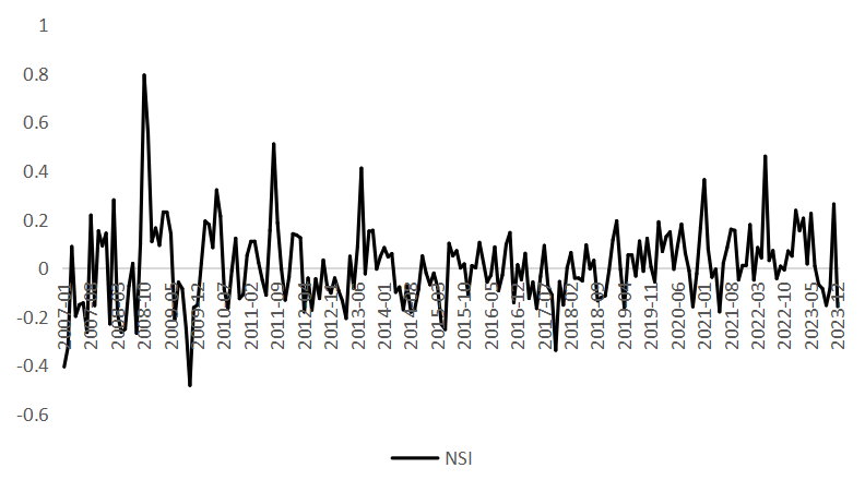
This study measures economic agents’ perception of financial risk using text mining techniques, referencing the methodology of Fan [28]. Keywords such as “financial market,” “financial industry,” “banking sector,” “capital market,” and “macroeconomy” are used to retrieve 38,728 relevant news articles from January 2007 to December 2024 via the CNKI newspaper database. Each news article is sentiment-scored using the SnowNLP library. To assess the importance of each newspaper, total number of articles, total downloads, and total citations are taken into account. The attention level of each individual article is measured by its download count and citation frequency. A Principal Component Analysis (PCA) is applied to calculate the attention weight of each article. Considering the variance in media attention across years, the attention score for each article is normalized by dividing its download and citation counts by the total download and citation counts of all articles in the same year. The final score for each article is obtained by multiplying its sentiment score by its attention weight. The monthly average score of all articles then constitutes the National Sentiment Index, which reflects the public’s perception of economic and financial risks. The sentiment trend is illustrated in Figure 1.

2.2.3. Construction of the macroeconomic index

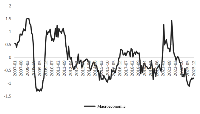
Following Ouyang Zisheng et al. (2019) [19], this study constructs a composite macroeconomic index based on key indicators of economic activity. These include the coincident index of macroeconomic prosperity, YoY growth of industrial added value above designated size, fixed asset investment, PMI, imports and exports, CPI, and PPI. These indicators comprehensively describe the macroeconomy across dimensions such as production, consumption, investment, prices, and trade. Principal Component Analysis (PCA) is used to synthesize these eight monthly indicators into a single composite macroeconomic index, which serves as a robust representation of the overall performance of China’s economy. The trend of this index is shown in Figure 2.

3. Empirical results and analysis

3.1. Impact of risks from financial markets on the macroeconomy

3.1.1. Evaluation of quantile model superiority

To more comprehensively validate the performance and reliability of the quantile XGBoost model, this study selects the Quantile Random Forest (QRF) model adopted by Duan et al. [29] as a benchmark. The evaluation metrics include Mean Absolute Error (MAE), Root Mean Squared Error (RMSE), and Coefficient of Determination (R²).

As shown in Table 2, both the QRF and quantile XGBoost models demonstrate improved overall performance after feature selection. However, when capturing tail characteristics of the distribution, the quantile XGBoost model exhibits lower MAE and RMSE and higher R² compared to the QRF, suggesting that the gradient boosting framework in XGBoost offers stronger nonlinear characterization of extreme values. In contrast, the QRF performs better around the median distribution (0.5 quantile), likely due to its theoretical unbiasedness in estimating conditional medians via direct optimization of the quantile loss function. Therefore, the quantile XGBoost model proves more advantageous in tail risk prediction. Based on this, we further employ the SHAP model to interpret the results of quantile XGBoost across different quantile levels.

3.1.2. Global and local SHAP interpretations

(1) Global Interpretability Analysis

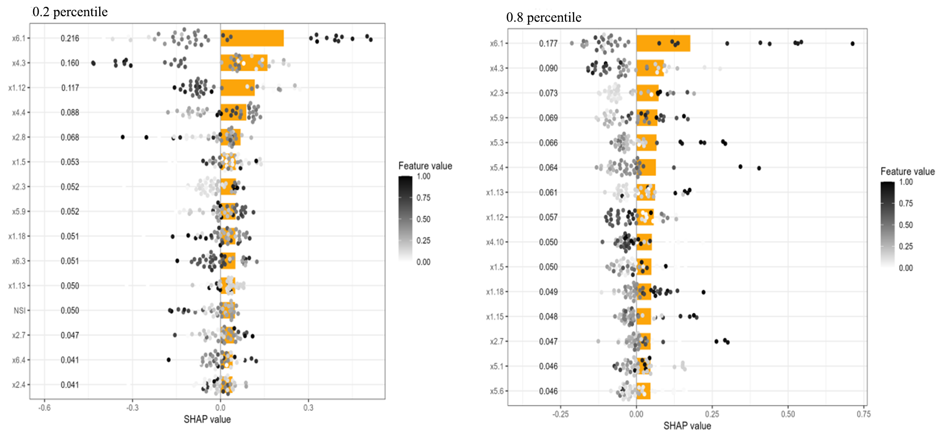
As illustrated in Figure 3, SHAP-based global interpretability reveals distinct risk factor contributions to macroeconomic conditions across distribution tails. Real estate development loan YoY growth (x6.1) consistently ranks as the most influential feature across both the upper and lower tails (SHAP values of 0.216 and 0.177, respectively). Its concentration in the positive SHAP region highlights a non-symmetric amplification mechanism—real estate investment acts as a financial accelerator for economic growth. ChinaBond Wealth Index YoY (x4.3), a proxy for liquidity in the fixed income market, ranks second across tails (SHAP values: 0.09/0.16). Its SHAP values span both positive and negative ranges, indicating a complex influence on economic performance. A divergence appears in the third-ranked variables: In the upper tail, price-to-book ratio of Wind300 ex-financials (x2.3) contributes positively to economic growth. In the lower tail, bank leverage ratio (x1.12) exhibits a one-sided negative SHAP distribution, suggesting a risk-amplifying role of financial leverage during downturns. Overall, factors such as real estate investment remain persistently important. During boom periods (upper tail), capital flows in the foreign exchange market (e.g., reserve growth, FDI growth) serve as key drivers. In contrast, during downturns (lower tail), macroeconomic stability becomes more dependent on financial market resilience—especially the dual constraints of bank leverage and bond market price signals.

(2) Partial Dependence SHAP Analysis (Feature-Level Interactions)

To further explore how national sentiment (NSI) interacts with key macroeconomic drivers across quantiles, we conduct SHAP dependence analysis between NSI and the top three features at the upper and lower tails.

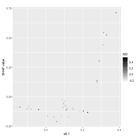
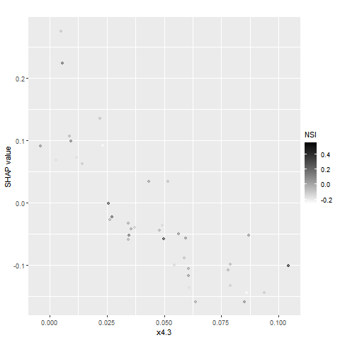
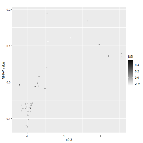
Figure 4. SHAP dependence plot – quantile 0.8

At the 0.8 quantile, NSI exhibits threshold-dependent marginal effects on major features: x6.1 (real estate loan YoY) shows a dual-threshold nonlinear response. Below 0.2, its contribution is marginal and mostly negative. Above 0.2, high NSI significantly enhances its positive marginal impact (SHAP increases by 35–40%), forming a synergy between real financing and optimistic expectations. x4.3 (bond wealth index) remains predominantly negative regardless of NSI, indicating a negative coordination. x2.3 (price-to-book ratio) contributes negatively when <3, but shifts to a positive driver when >3, especially in tandem with high NSI, signaling a joint pro-cyclical impact of valuation and confidence.

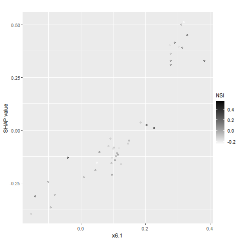
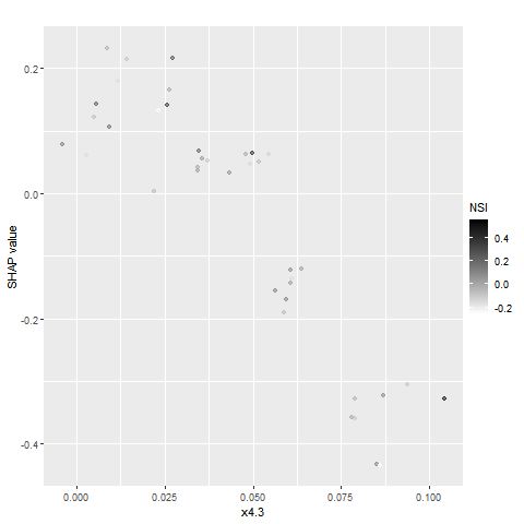
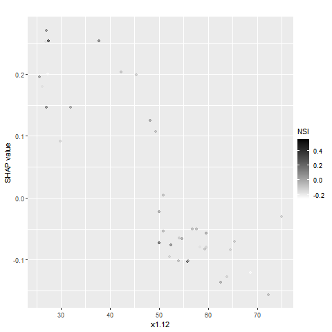
Figure 5. SHAP dependence plot – quantile 0.2

According to Figure 5, at the 0.2 quantile: As x6.1 increases, representing more active real estate investment, it co-varies positively with NSI. When x6.1 exceeds 0.2, the coupling of vibrant markets and improved sentiment boosts macroeconomic expansion. x4.3, representing bond market stability, exerts a positive impact under low volatility and high NSI—indicating that lower price fluctuations help stabilize asset valuation expectations and facilitate fixed income–real economy transmission. x1.12 (bank leverage ratio) in the moderate range (20–50), combined with high NSI, promotes economic growth. This suggests that moderate leverage, together with sentiment resonance, enhances credit elasticity and efficient financial resource allocation.

(3) Characterization of Extreme Events

This paper selects the period of the 2008 financial crisis from the macroeconomic index chart as a case of extreme events for upper-tail and lower-tail analysis.

In the upper-tail distribution, the impact of extreme financial risk events is manifested during the period from September 2008 to January 2009, when China's macroeconomic index fell below the critical threshold and continued to decline. Within the financial market, a risk resonance was observed between the sharp volatility of the ChinaBond Composite Index (x4.3) and the negative deviation of the FR007-based interest rate swap (x4.4). The cumulative maximum loss (CMAX) of the financial sector stock index (x1.15) made a significant negative contribution. In the real estate market, the year-on-year growth rate of completed real estate investment (x6.1) contracted, while FDI growth (x5.4) deviated negatively, jointly constituting critical constraints that triggered a precipitous drop in real estate investment, with growth plummeting by 12.7%. Simultaneously, the rise in the central tendency of the 7-day interbank repo fixing rate (x3.1) increased short-term funding strain on the real economy. Increased exchange rate volatility amplified external shocks through capital flow channels, while rising stock market risk premiums further weakened the wealth effect.

From July 2009 to January 2010, China’s macroeconomic index turned positive and began to rise. The year-on-year growth of completed real estate investment (x6.1) contributed +0.296, combined with a sustained positive contribution from sector indicators (x6.3), highlighting the stimulative financing effects of the central bank’s policies—lowering the reserve requirement ratio and offering mortgage rate discounts. The year-on-year growth of FDI (x5.4) contributed +0.245, indicating an improved balance of payments due to increased external capital inflows. The share of medium- and long-term loans (x1.5) contributed +0.121, suggesting that optimization of the financial structure enhanced resource allocation efficiency, and reflecting the effectiveness of the RMB 4 trillion stimulus package. The spread between the 3-month interbank offered rate and the fixed deposit rate (x1.18) made a positive contribution, reflecting enhanced liquidity in the financial market, thus providing a stable environment for real-economy financing. The composite index rose from -0.518 to +0.619, signaling the emergence of synergistic effects from multi-objective policy coordination. See Figure 6 for details:

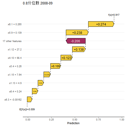
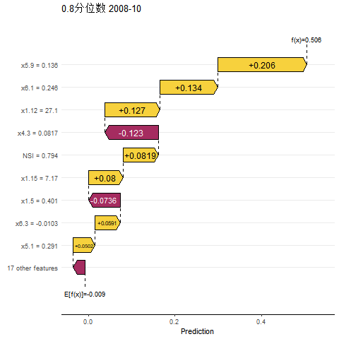
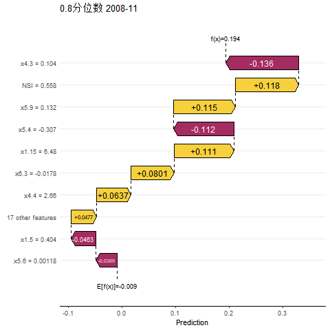
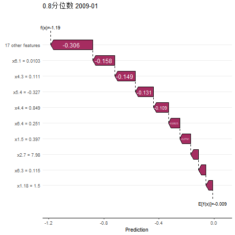
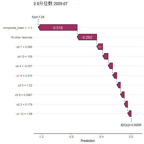
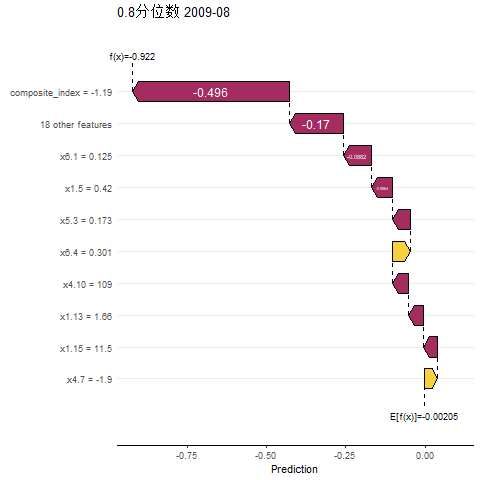
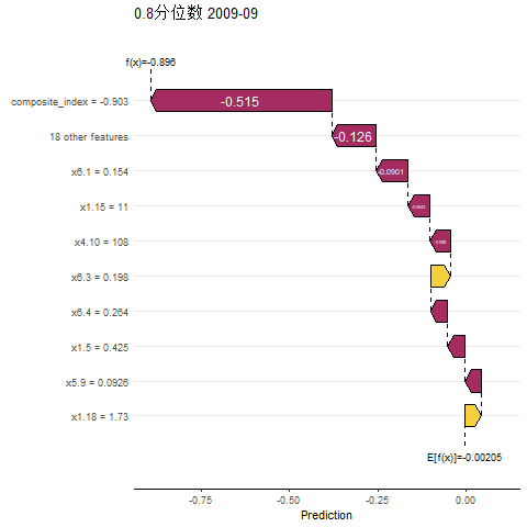
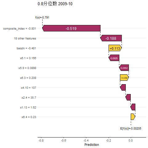
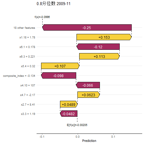
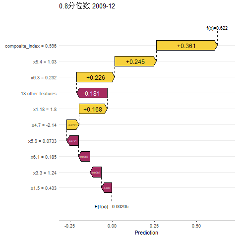
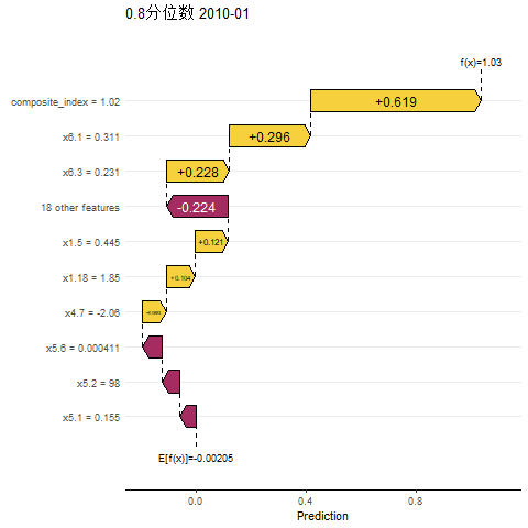
Figure 6. Illustration of extreme events (upper tail)

In the lower-tail distribution, the impact of extreme financial risk events was also concentrated in the September 2008 to January 2009 period, during which China’s macroeconomic index fell below the critical threshold and continued downward. The negative contribution of the ChinaBond Composite Index (x4.3) was significant (from -0.331 to -0.278), while the contribution of FDI growth (x5.4) sharply declined to -0.327, highlighting the withdrawal of international capital from the Chinese market as the crisis deepened. Other indicators, such as the financial market liquidity indicator (x1.18), also gradually made negative contributions, forming a risk resonance.

During the recovery period from July 2009 to January 2010, China’s macroeconomic index turned positive and began to rise, with key drivers exhibiting clear signs of policy response. The +0.3 positive contribution (January 2010) from the year-on-year growth in completed real estate investment (x6.1) underscored the targeted easing in the real estate sector under the RMB 4 trillion stimulus package, stimulating a rebound in real estate investment momentum. The improvement in credit structure was reflected in the steady rise in the share of medium- and long-term loans (x1.5) (from +0.0938 to +0.271), indicating a growing willingness for long-term investment in the real economy. Among the supporting factors, the decline in exchange rate volatility (x5.9) and the coordinated improvement of multiple indicators (17 other features, combined contribution +0.15) further strengthened the synergy between external environment stability and domestic demand recovery. See Figure 7 for details:

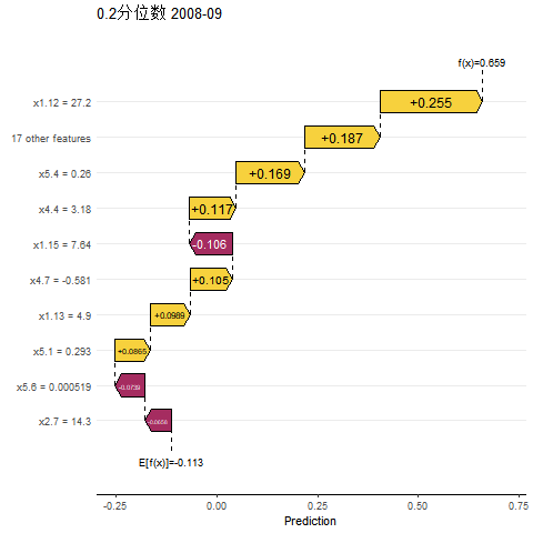
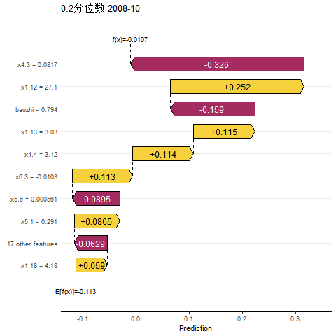
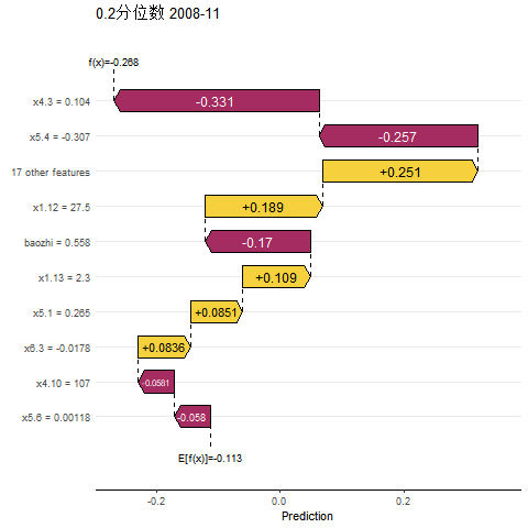
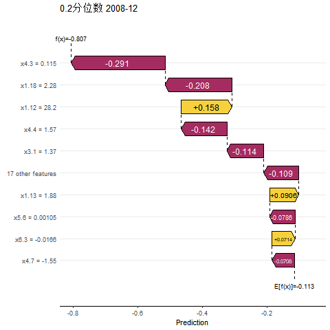
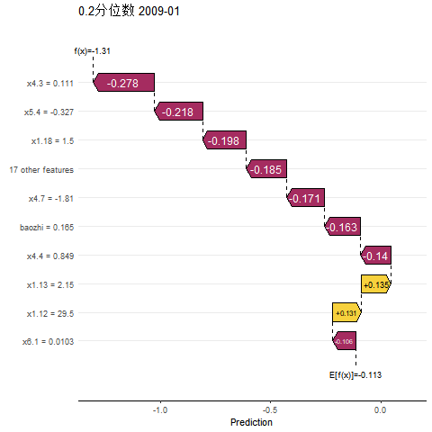
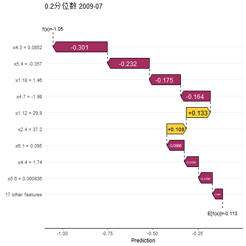
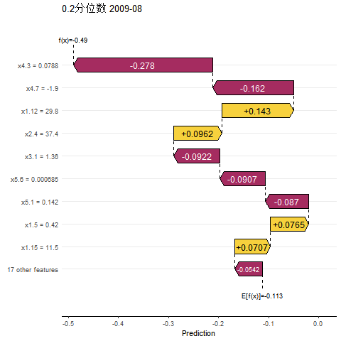
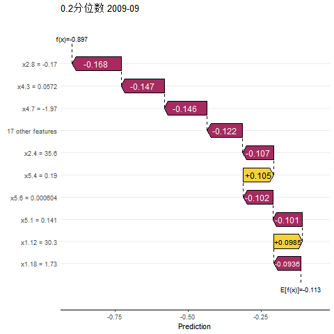
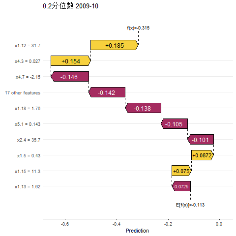
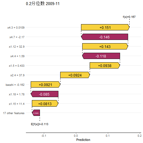
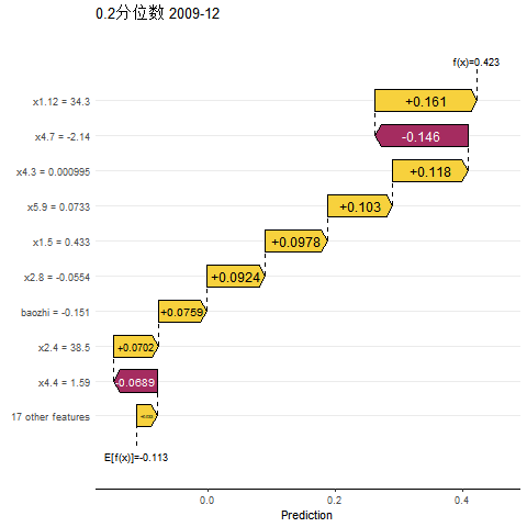
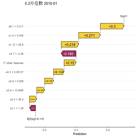
Figure 7. Partial SHAP analysis of extreme events (lower tail)

In summary, the quantile framework reveals asymmetric characteristics in macroeconomic performance during 2008–2010. During the crisis period (2008–2009), quantile heterogeneity displayed significant differences in risk transmission: In the upper tail, the year-on-year growth of real estate investment (x6.1) served as the dominant driver, transmitting shocks along the industrial chain to the meso-level sector. At the 0.2 quantile in the lower tail, the sharp drop in FDI (x5.4) and the ChinaBond Composite Index (x4.3), coupled with worsening liquidity indicators (x1.18), produced compounded effects. During the recovery phase (July 2009 to January 2010), quantile heterogeneity evolved into a structural transformation of growth drivers: At the upper 0.8 quantile, the growth continued to be driven by the real estate and FDI sectors. At the lower 0.2 quantile, recovery was first led by improvements in bank leverage (x1.12) and credit structure (x1.5), indicating that extremely depressed conditions rely more on the endogenous recovery capacity of the financial system.

3.2. Tail risk spillover analysis

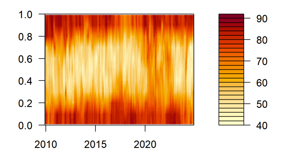
To further investigate the dynamic transmission mechanisms of financial risks, this study utilizes the Kernel Principal Component Analysis (KPCA) method. By employing nonlinear mapping principles, we construct composite indices that capture significant nonlinear characteristics across different market dimensions, effectively uncovering complex interactions and deep structural relationships within the data. Based on this, we apply the QVAR-DY model to analyze the risk spillover effects between various financial market dimensions and the macroeconomy from both static and dynamic perspectives. The static analysis examines the spillover effects across different tail distributions, while the dynamic analysis uses a rolling time window to track the time-varying characteristics and evolution paths of risk transmission, offering a more comprehensive understanding of the dynamic spillovers between financial markets and the macroeconomic environment. According to the total spillover index across different quantiles (Figure 8), the overall spillover level of the system is significantly higher in the tail distributions. Specifically, the 0.8 and 0.2 quantiles are identified as critical thresholds for extreme risk spillovers. Conducting risk spillover analysis at these quantiles is more conducive to identifying the triggers of systemic tail risk.

3.2.1. Static analysis of tail risk spillovers

(1) Spillover Effects under the Median Distribution

According to the static spillover table at the median distribution (Table 3), under normal market conditions: First, the total spillover (TO) across markets amounts to 83.69. The stock market (SM) contributes the highest spillover at 20.00, followed by the bond market (BM) at 16.85, both exhibiting strong outward spillover effects. In contrast, the bond market also receives significant spillover from others, with a high FROM value of 19.05, whereas the real estate market (REM) is less affected, with a FROM value of only 4.67. Second, in terms of net spillover (NET), the stock market (SM) and real estate market (REM) are net transmitters of risk, playing a contributory role in the propagation of financial instability. Meanwhile, macroeconomic indicators (MI) and national sentiment index (NSI) are net receivers of risk, suggesting greater vulnerability to external shocks. Finally, examining specific markets: the stock market's high TO value reflects its strong shock impact on other markets; the bond market's high FROM value indicates its susceptibility to external influences. The financial institutions market (FIM) shows moderate outward spillover (TO = 7.41) but is also relatively sensitive to other markets (FROM = 13.72).

(2) Spillover Effects under the Upper Tail Distribution (0.8 Quantile)

As shown in the static spillover table at the 0.8 quantile (Table 4), under bullish market conditions: First, the total spillover (TO) across markets surges to 289.74. The financial market (FM) demonstrates the strongest outward spillover at 58.59, followed by the national sentiment index (NSI) at 40.01. In contrast, the financial institutions (FIM) and bond market (BM) show relatively weaker spillover effects. From the perspective of risk absorption (FROM), the money market (MM) and bond market (BM) exhibit high vulnerability to shocks, with FROM values of 45.79 and 45.56, respectively. The real estate market (REM), however, remains relatively unaffected (FROM = 8.51). Second, in terms of net spillovers, the financial market (FM) and real estate market (REM) are net risk exporters, while financial institutions (FIM), bond market (BM), money market (MM), stock market (SM), and national sentiment index (NSI) are net importers, indicating a higher susceptibility to risk contagion. Finally, the financial market (FM) not only shows the highest TO, reinforcing its strong influence across other sectors, but the real estate market (REM), despite a low FROM, shows a considerable TO of 25.02—suggesting it cannot be overlooked in systemic risk transmission.

The static spillover table at the 0.2 quantile (Table 5) reflects conditions in a bearish market: First, the total spillover (TO) reaches its highest level at 290.91, indicating intensified systemic risk during market downturns. The stock market (SM) emerges as a key transmitter with a TO of 48.23. Financial institutions (FIM) and the money market (MM) show moderate outward spillovers, while all other sectors contribute to varying degrees. From the perspective of spillover reception, the stock market (SM) (FROM = 47.31) and macroeconomic indicators (MI) (FROM = 46.75) are most affected. In contrast, the real estate market (REM) (FROM = 18.11) and money market (MM) (FROM = 23.96) remain relatively insulated. Second, in terms of net spillovers, the real estate market (REM), money market (MM), stock market (SM), and national sentiment index (NSI) are net exporters, suggesting active roles in transmitting risk under stress. Lastly, the high TO value (48.23) and slightly positive NET (0.92) of the stock market (SM) point to its potential as a primary initiator of cross-market risk contagion. The high FROM values of SM and MI reflect their strong exposure to external shocks. The REM's low FROM but high TO (41.91) underlines its significant influence on other sectors, despite limited susceptibility.

In summary, the financial institutions sector (FIM) consistently exhibits relatively high spillover (TO) across quantiles, underlining its critical role in cross-market risk transmission. Risk interactions are active across all quantiles, but spillovers peak under bearish conditions (0.2 quantile), where total outward spillover reaches 290.91. This suggests that during market downturns, risk contagion becomes more widespread and intense. Such periods often trigger investor panic, liquidity shortages, and systemic instability—making it easier for volatility in one sector to propagate rapidly across multiple markets, thereby amplifying total systemic risk.

3.2.2. Dynamic analysis of tail risk spillover

While static spillover effects can reveal the intensity and direction of spillovers between market dimensions and the macroeconomy, they cannot capture the time-varying characteristics of spillovers between markets, especially under the influence of extreme events, when spillover levels may fluctuate significantly. Referring to Huang Botao et al. (2024) [31] and Tiwari et al. (2018) [32], and considering the presence of a first-order lag in the data, this study sets the rolling window length to 37 months (one month longer than 36) to capture dynamic changes in risk spillovers under different economic and financial environments.

(1) Dynamic Total Risk Spillover

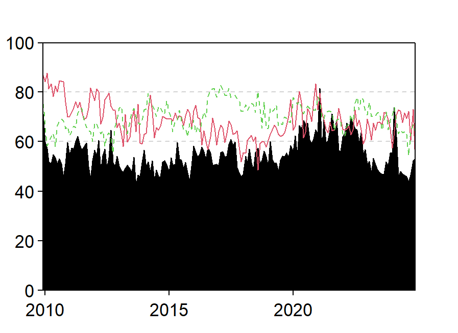
As shown in Figure 9, the total risk spillover effects between the macroeconomy and various market dimensions exhibit pronounced time-varying features in both the upper tail and lower tail distributions. At the 0.8 quantile (solid line), the total spillover level outside the rolling window fluctuates between 40% and 85%. At the 0.2 quantile (dashed line), the total spillover level similarly fluctuates between 50% and 85%, with comparable ranges of volatility. This suggests that high-frequency risk transmission is triggered in both lower and upper tails. Under normal conditions (shaded area), total spillover levels are relatively lower compared to tail risk spillovers (solid line for upper tail, dashed line for lower tail). The total spillover at the 0.8 quantile experiences more intense fluctuations during sudden major events (e.g., the 2015 stock market crash and the 2020 COVID-19 pandemic) than at the 0.2 quantile. Hence, risk spillovers at the 0.8 quantile tend to reflect rapid surges and quick declines in spillover levels triggered by such events, indicating that risk transmission during extreme events is stronger and faster than during normal periods, with market risks quickly accumulating and dissipating in the short term. By contrast, the fluctuations at the 0.2 quantile are relatively stable and high-frequency, reflecting the market's passive response to long-term adverse factors and the gradual release of risks under negative conditions.

(2) Dynamic Net Spillover between the Macroeconomy and Market Dimensions

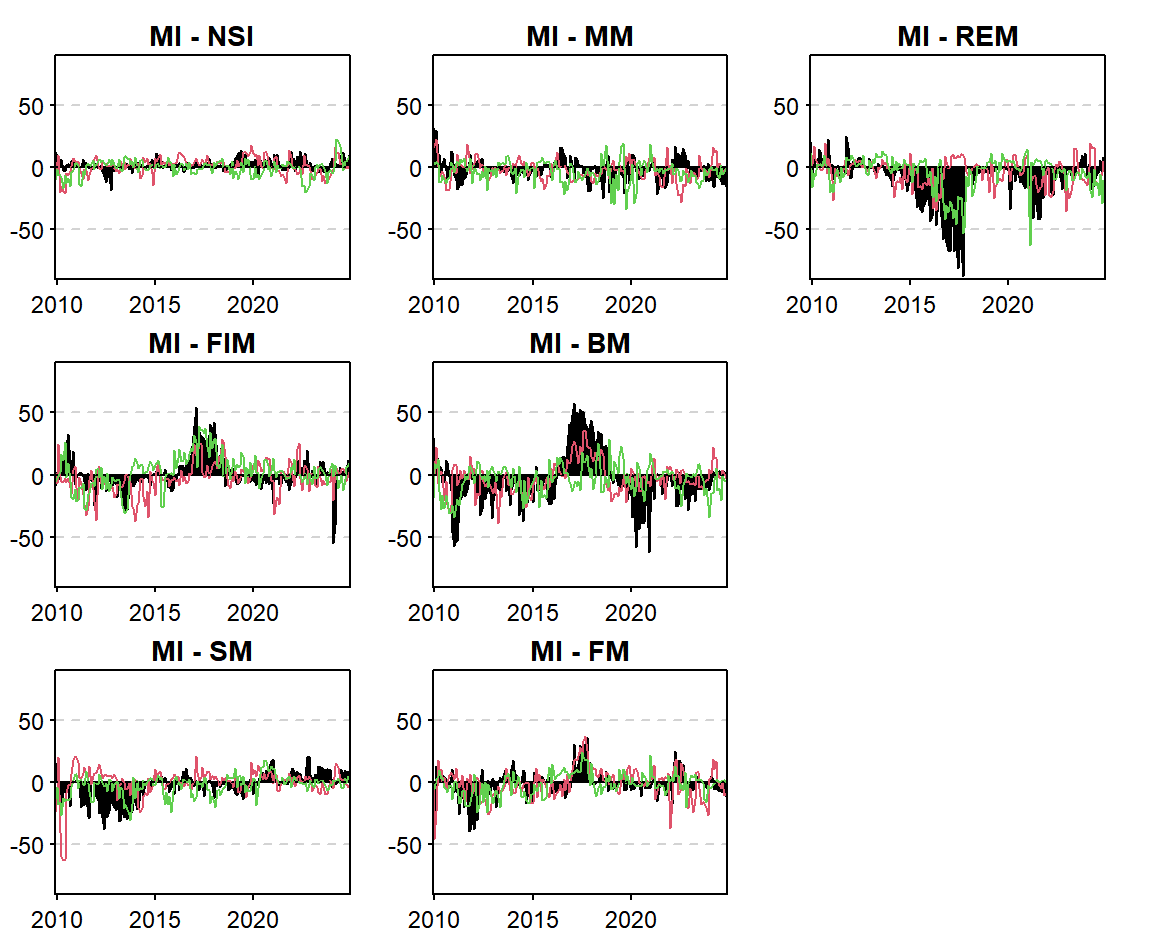
Overall, the net spillover effect from the macroeconomy (MI) to seven market dimensions—including national sentiment (NSI), financial institutions (FIM), stock market (SM), money market (MM), bond market (BM), foreign exchange market (FM), and real estate market (REM)—exhibits significant asymmetry and event-driven characteristics. At the 0.8 quantile (red line), risk transmission demonstrates an “event-driven—mechanism amplification” explosive pattern, whereas at the 0.2 quantile (green line), policies and reforms act as a “risk buffer,” smoothing volatility.

At the 0.8 quantile, the red line peaks higher than the green line at specific time points, illustrating that extreme events serve as catalysts for risk transmission. For example, during the 2015 stock market crash, large-scale deleveraging of leveraged stock funds triggered market panic, causing MI’s net spillover to the stock market to surge to a peak at the 0.8 quantile. This reflects how economic expectation fluctuations were amplified via leverage mechanisms into violent market shocks. Similarly, during the 2020 COVID-19 pandemic, MI’s net spillover to national sentiment increased significantly, highlighting the negative feedback loop formed between economic downturn pressure and public pessimism, which intensified risk contagion.

In contrast, the net spillover at the 0.2 quantile fluctuates more moderately, highlighting the stabilizing effects of policy interventions and structural reforms. For instance, during the 2016 monetary easing cycle, MI’s net spillover to the money market was negative, indicating that liquidity easing effectively supported the real economy and weakened market risk linkages.

At the 0.5 quantile, representing a neutral market expectation state (neither highly optimistic nor extremely pessimistic), the relationships between dimensions show different degrees of extreme spillover or spill-in after major crises such as the 2008 financial crisis, 2015 stock market crash, and 2020 pandemic. This uncertainty leads to cautious investor decisions sensitive to short-term information, thereby intensifying risk transmission.

(3) Dynamic Analysis of Net Spillover Networks

① Network Dynamics under Normal Conditions

In net spillover network graphs, red nodes represent positive net spillover (net transmitters), green nodes represent negative net spillover (net receivers), node size reflects the magnitude of spillover or spill-in, and the proximity between nodes indicates the closeness of their connections. This visualization intuitively presents the direction, strength, and interrelationships of risk net spillovers among market dimensions under different distributions, providing a clear perspective for understanding the risk transmission mechanism between the macroeconomy and markets.

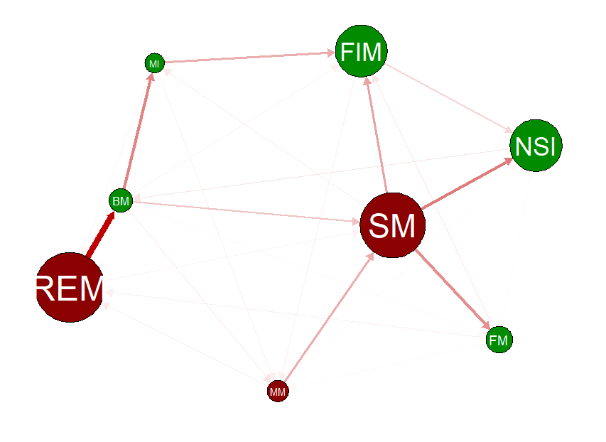
As shown in Figure 11, under normal market conditions (0.5 quantile), the main risk transmitters ranked by spillover magnitude are REM (real estate), SM (stock market), and MM (money market). REM and BM (bond market) are closely linked, suggesting that volatility in the real estate market easily transmits to the bond market. SM is the core spillover source, strongly connected to FIM (financial institutions), NSI (national sentiment), and FM (foreign exchange), implying that stock market performance significantly influences financial institutions, public sentiment, and the forex market. MM’s overall spillover volume is relatively limited, indicating its spillover effect is not prominent under normal conditions. MI (macroeconomy) appears as the smallest green node, implying its stability and relatively minor influence from other market dimensions during normal periods.

② Network Dynamics under Tail Conditions

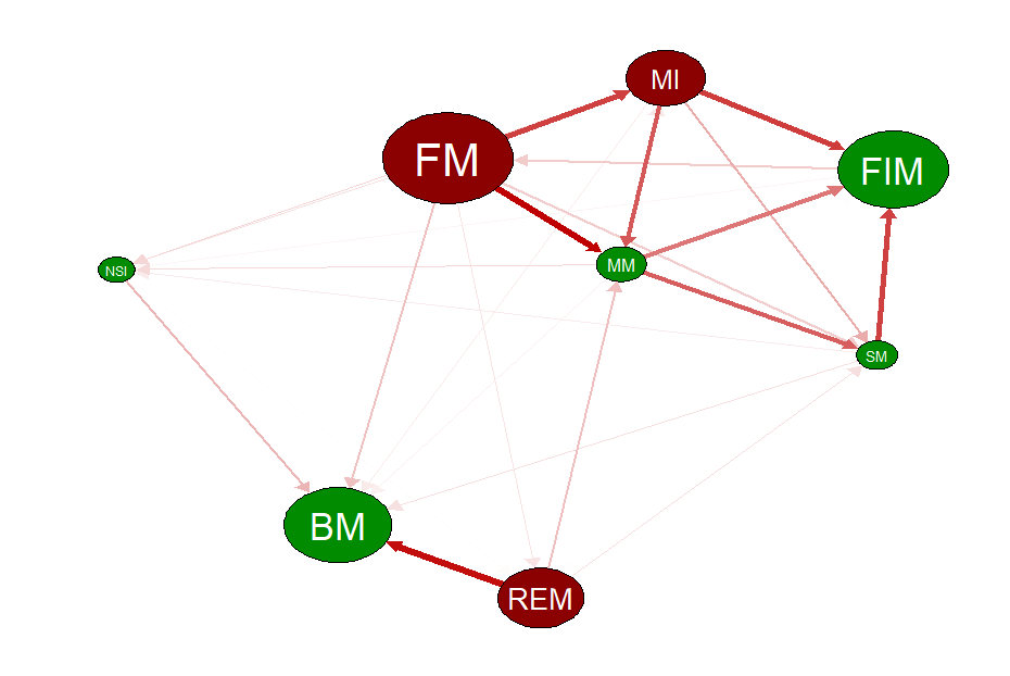
Figure 12 shows that under positive market conditions (upper tail 0.8 quantile), the main risk transmitters ranked by spillover size are FM (foreign exchange), REM (real estate), and MI (macroeconomy). FM is closely connected with MI, MM, and SM, indicating that in bullish markets, the activity of the forex market requires close monitoring to prevent potential risks to China’s macroeconomic and monetary stability. REM shows significant spillover to BM, implying that real estate volatility transmits to bonds, potentially via capital allocation or market confidence. MI’s role as a risk transmitter under favorable conditions is also evident. NSI exhibits negative net spillover and weak connections with other dimensions, indicating limited influence from and to other markets during macroeconomic upturns.

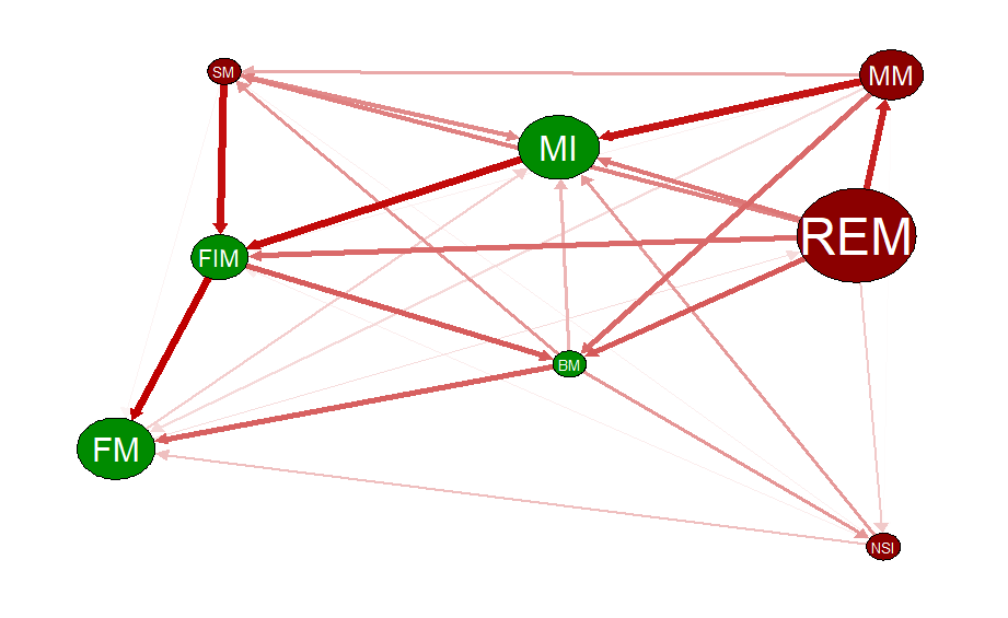
According to Figure 13, under bearish market conditions (lower tail 0.2 quantile), the primary risk transmitters ranked by spillover magnitude are REM (real estate), MM (money market), SM (stock market), and NSI (national sentiment). The strong spillover chains REM → MM → MI and SM → FIM reveal core pathways of risk transmission under specific market conditions. This indicates that fluctuations in the real estate market significantly impact the money market, which then affects macroeconomic operations. Meanwhile, a depressed stock market directly threatens financial institutions’ stability, highlighting the hierarchical and tightly connected nature of risk transmission within the economic-financial system. This analysis offers valuable insights into systemic risk propagation mechanisms and underscores the importance of monitoring these critical pathways during market downturns to prevent risk contagion.

Comparing across states, under normal conditions, REM and BM form a small risk cluster. In bullish markets, besides the REM-BM cluster, FM, MI, FIM, MM, and SM form an additional risk spillover cluster. In bearish markets, risk clustering and spillover intensity across all market dimensions are the most pronounced.

4. Research conclusions and policy recommendations

To deeply characterize and analyze the tail risk factors and the static and dynamic risk spillover effects among various financial sub-markets, national sentiment, and the macroeconomy, this study selects 66 basic indicators across seven dimensions: financial institutions, stocks, money market, bonds, foreign exchange, real estate, and national sentiment. Given the high dimensionality, information redundancy, and nonlinearity of these indicators, the study first applies the RReliefF-RF-RFE method for feature selection. Then, it uses quantile XGBoost combined with SHAP for interpretation, analyzing the impact of risk factors across different quantiles on China’s macroeconomic operations from January 2007 to December 2024. Finally, nonlinear dimensionality reduction is performed via Kernel Principal Component Analysis (KPCA) on the selected feature space to synthesize composite indices for each dimension while preserving dynamic coupling characteristics. A time-varying parameter Quantile Vector Autoregression-Dynamic (QVAR-DY) model is constructed to further explore the static and dynamic multidimensional risk spillover effects of systemic financial risk. The main findings are:

First: Under different tail states of macroeconomic operation, the year-on-year growth rate of real estate development loans and the ChinaBond Composite Index Wealth Index are identified as core risk factors. However, other risk factors exhibit significant heterogeneity. National sentiment shows significant synergistic and threshold effects on key macroeconomic features. In the upper tail state, national sentiment amplifies expectations and synergizes with factors such as real estate development loans and price-to-book ratio, jointly driving economic growth. In the lower tail state, national sentiment positively couples with real estate investment, bond market stability, and moderate bank leverage, promoting economic system recovery by stabilizing market confidence and asset valuation expectations. This indicates a dynamic interactive relationship between market states, core economic variables, and national sentiment, jointly influencing macroeconomic operation.

Second: Based on the static analysis of tail risk spillover, the comprehensive risk spillover value is highest in the lower tail state, with significantly enhanced financial risk linkage across dimensions. In normal states, stocks and bonds exhibit prominent risk spillover capabilities, while the macroeconomy and national sentiment are more vulnerable to shocks. In bullish markets, the financial market and national sentiment dominate risk spillover, with the money market and bond market more susceptible to contagion and becoming net risk recipients across multiple markets. During market downturns, the stock market leads in spillover intensity, with real estate and other markets acting as primary net risk transmitters, resulting in the most intense risk transmission.

Third: From the dynamic analysis of tail risk spillover, risk spillover in the upper tail mostly manifests as sharp surges and rapid declines during event occurrences, indicating that under extreme events, risk transmission intensity and speed far exceed those in normal periods, with market risk quickly accumulating and releasing in the short term. The lower tail risk spillover exhibits relatively stable, high-frequency fluctuations, reflecting the market’s passive response to long-term adverse factors and gradual risk release under negative environments. Under normal market conditions, the real estate and bond dimensions form a small risk cluster. In the upper tail (bullish) state, besides the real estate and bond cluster, the foreign exchange, macroeconomic, financial institutions, money market, and stock dimensions also form a risk spillover cluster. In the lower tail (bearish) state, risk clustering and spillover intensity across all dimensions are most pronounced. This spillover transmission provides empirical support for relevant departments in formulating risk prevention measures.

Based on the conclusion above, this paper proposes the following recommendations:

First: Strengthen cross-departmental coordination mechanisms and establish dynamic interdepartmental monitoring systems to guide market expectation management. Relevant authorities should build a macroeconomic monitoring framework centered on core influencing factors, combined with changes in national sentiment indices, to track key drivers of economic operation under different tail states in real-time. This will enable dynamic capture and early warning of the nonlinear features of the macroeconomy and rational guidance of market expectations—preventing excessive speculation in bullish markets and boosting market confidence to avoid panic during downturns.

Second: Implement differentiated regulatory strategies, improve risk isolation mechanisms, and optimize market information disclosure. Based on risk transmission characteristics in various market states, focus regulation on risk spillovers between the stock and bond markets during normal states, strictly regulating trading behavior. In bullish markets, strengthen monitoring of fluctuations in financial markets and national sentiment. In bearish markets, enhance supervision of the stock and real estate markets to prevent excessive risk propagation. For markets that are net risk recipients, establish risk buffers and isolation systems, such as special risk reserves and restrictions on disorderly cross-market capital flows, to reduce the impact of external risk shocks. Increase transparency across financial markets, especially during tail states, by timely and accurately disclosing risk-related data to reduce information asymmetry and prevent irrational investor behavior, thus lowering uncertainty in risk transmission.

Third: Develop tiered emergency response plans, strengthen risk prevention in key dimensions, and promote interconnected regulation of financial markets. In response to the rapid accumulation and release of risks during upper-tail extreme events and the gradual impact of long-term adverse factors in the lower tail, establish tiered emergency response mechanisms that clarify responsible entities, handling procedures, and policy tools under different risk states to ensure quick and effective responses. Given the changes in risk spillover clusters under various market conditions, break down regulatory barriers to create unified cross-market and cross-dimensional regulatory coordination mechanisms. Enhance monitoring and analysis of capital flows and market linkages to improve overall financial market risk prevention capabilities.