

1. Introduction
The Transportation system is a fundamental aspect of urban life that intimately affects the populace. An excellent transportation system can facilitate people's movement and enable individuals to access various places more easily, such as companies, schools, and shops. Transportation also plays a major role in economic development. Additionally, such a transportation system can also increase the flow of people in the business district, which can promote consumption. There are various types of transportation and taxi is one essential part among them. Taxis have played an important role since ancient times, and they evolved from horse-drawn carriages to automobiles. Now, online car-hailing has become the main form of taxi. It allows people to order a trip more conveniently at any place. People can see the predicted price directly after they enter the locations in some taxi applications such as Uber and Lyft. With this information, people can make a better schedule for their travel plans. Thus, increasing the prediction accuracy of fares is of great importance.
However, taxi fares are difficult to predict precisely, especially in some metropolitan cities such as New York City. They are affected by several factors like travel distance, traffic conditions, weather, and temporal factors [1]. The variability of these factors over time further complicates the task of identifying an accurate relationship between fare and these variables. Hence, finding the accurate relationship between fare and these factors is challenging. To address this challenge, various companies and researchers utilize distinct prediction models that account for different factors, such as travel distance, the number of passengers, and the time of the trip. However, the accuracy of the model is not enough and still needs to be improved. An inaccurate prediction is likely to force passengers to pay more than the actual taxi fare, which should be solved by machine learning.
Machine learning is a subset of artificial intelligence and it is a good tool for building models to train and test a huge dataset based on various algorithms [2]. This technology can be used in various areas such as finance and healthcare. Its main objective is to find the relationship between variables so that it is able to predict the target value [3]. Machine learning can be mainly divided into two types which are supervised learning and unsupervised learning [3]. The main difference between these two is that supervised learning trained models based on a labeled data subset while unsupervised learning not [4]. In this paper, supervised learning was used to predict the taxi fare in New York City. It has the regression algorithms which can be used to predict the unknown variables and it suits the best as per the requirement of predictive analysis [2,5]. There are three prediction models in total: Linear regression model, decision tree model, and random forest model. In these three models, the taxi fare was predicted based on the following variables: distance between pickup and drop off location and number of passengers. This research aims to find the best one among these three models.
2. Method
2.1. Data preparation
This article used data from Kaggle which contains about 55 millions rows data [6]. Each row consists of six features such as pickup_longitude and pickup_latitude. The objective of this dataset is to use machine learning models to predict the amount of fare for each taxi ride. The model in this paper read 100,000 rows of original data.
Prior to training the model, a crucial stage is preprocessing of the original data. The first step involves calculating the distance between pickup location and drop off location. This article used the haversine formula which gives minimum distance between the two locations on a spherical body based on latitudes and longitudes [7].
\( d=2×R×arcsin(\sqrt[]{{sin^{2}}(Δlatitude/2)+cos(lat1)×cos(lat2)×{sin^{2}}(Δlongitude/2)} ) \) (1)
\( Δlatitude=lat1-lat2 (difference of latitude) \) (2)
\( Δlongitude=lon1-lon2(difference of longitude) \) (3)
Where R is the radius of earth (6371 km). d is the distance computed between two points. Next step is data cleaning. In the dataset, some values are obviously wrong and should not be used. This process deletes the data that occurs in the following 4 conditions:
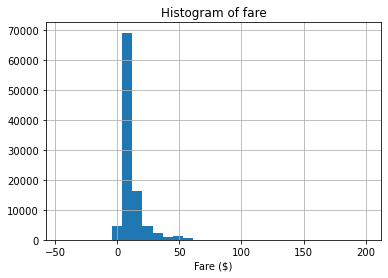
Figure 1. The histogram of fare.
From the histogram of fare (Figure 1), some values are negative. In reality, it is impossible for passengers to pay a negative price. Thus, these data should be removed.
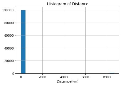
Figure 2. The histogram of distance.
From the histogram of distance (Figure 2), there are some values over 8000 km which are highly possible wrong. Hence, these data also should be removed.
Table 1. Examples of some location data. | ||||
pickup_longitude | pickup_latitude | dropoff_longitude | dropoff_latitude | distance |
-74.6898 | 40.1906 | -74.6898 | 40.1906 | 0 |
-74.4293 | 40.5 | -74.4293 | 40.5 | 0 |
-74.1829 | 40.7176 | -74.1829 | 40.7176 | 0 |
0 | 0 | 0 | 0 | 0 |
0 | 0 | 0 | 0 | 0 |
From Table 1, the pickup and drop off locations of some data are exactly the same and the values of some data are all zero. Both will cause the distance to be zero. Remove these data.
Table 2. Examples of fare and distance. | |
fare_amount | distance |
3.7 | 129.95 |
4.1 | 129.56 |
7.7 | 127.199 |
From Table 2, some rows have a large distance value but only with a small fare. These data have a huge influence on the accuracy of machine learning models. The models in this article delete data with distance larger than 50 but with a fare smaller than 10. After preprocessing, there are 59069 rows of data remaining.
2.2. Machine learning models
Linear Regression. The initial model employed in this study to forecast fare is linear regression. This statistical technique holds a significant place in the analysis of the association between diverse variables [8]. The primary objective of this method is to predict the reliant variables, given the independent variables [9]. In this research, the closed-form solution of linear regression was applied to accomplish the regression analysis and obtained the desired output values.
In order to test the accuracy of the model, the total dataset after preprocessing was divided into the train set(i.e. X_train, Y_train) and the test set(i.e. X_test, Y_test) by using a function called train_test_split from sklearn.model_selection. Specifically, the train set was 80% and the test set was 20%.
This study chose multivariate linear regression. The two independent variables contained in this model are the distance and the number of passengers. X_train contains distance(first column) and number of passengers(second column). Y_train contains one column of fare. Before calculating the coefficients W, add one column of dummy variables 1 in X_train by using np.hstack. Then use the two train sets to train the model through closed_form formula.
Decision Tree. Decision tree is the second model used in this paper. It is one of the most effective methods for data mining. It can help develop prediction algorithms for the target variable [10]. This prediction model has many advantages. It can identify the features and extract patterns in a large database which are important for prediction [11]. In this paper, the maximum depth of the model is 3. X_train and Y_train are used to train the decision tree model by using model.fit(X_train, Y_train).
Random forest. Random forest is the third model which can also be used for regression analysis. It combined multiple decision tree predictors [12]. Each tree is based on the values of a random vector sampled independently and with the same distribution for all trees [12]. This type of model can make a more accurate prediction since the collection of trees is better than a single tree [2]. The model used RandomForestRegressor to set the maximum depth to be 3 which is the same as the previous decision tree model, and the n_estimater value is 80. Use X_train and Y_train to fit the model through code model.fit(X_train,Y_train).
The Root Mean Square Errors (RMSE) was employed to test the accuracy of the model performance. This criterion is a standard metric for model evaluations [13]. A smaller RMSE means a better prediction.
\( RMSE=\sqrt[]{\frac{1}{n}\sum _{i=1}^{n}e_{i}^{2}} \) (4)
3. Results and discussion
Table 3. Values of RMSE of each model. | |
Model | RMSE |
Linear Regression | 1.718 |
Decision tree | 1.277 |
Random forest | 1.264 |
Among these three models, the random forest model has the smallest root mean square error 1.264 and the linear regression model has the largest root mean square error 1.718 shown in Table 3. The decision tree model has an error of 1.277 which is a little bit larger than the random forest model. Thus, random forest is a more accurate machine learning model to predict the taxi fares in New York city. In addition, compared to the RMSE (1.470) of the random forest models mentioned in other research [2], this model has a relatively smaller error so that it can has a more accurate prediction.
4. Conclusion
This study proposes the application of supervised learning techniques to predict taxi fares in New York City. To achieve this objective, three machine learning models, including linear regression, decision tree, and random forest, were developed and evaluated based on the root mean square error metric. The findings reveal that the random forest model outperforms the other two models with the smallest error rate of 1.264. Accordingly, the random forest model is suggested as the most effective approach for the prediction of taxi fares in New York City. However, it is worth noting that the decision tree model also yielded a relatively small error rate of 1.277. Nevertheless, the current models have some limitations as they only consider the distance and the number of passengers in the prediction process, while other factors such as pickup time and traffic conditions can also affect the taxi fares. Hence, further research is recommended to incorporate additional variables and explore other machine learning models such as Gradient Boosting Regression that could enhance the accuracy of the prediction.