


1. Introduction
Breast cancer is one of primary malignancy of female and it is also an important cause of the death of female cancer patients [1]. The prediction of breast cancer is of great importance. Using machine learning techniques to predict and diagnose breast cancer has been a hot topic over the past few decades. In traditional diagnosis and treatment, doctors rely on visual acuity sensory information analysis imaging to determine the malignant degree of breast disease is not only time-consuming but also cannot guarantee the efficiency and accuracy of the diagnosis [1,2].
Nowadays, with the continuous development of machine learning, it has brought many conveniences to the field of medical and health care. Doctors use trained models to assist in diagnosing patients with cancer, improving work efficiency and diagnostic accuracy [3]. However, today's models have certain shortcomings, such as naive Bayesian algorithms, which must make the attribute conditional independence assumption, but nowadays data gets more and more, and get more complex, the true independent data is rare [4]. KNN algorithm has a low accuracy in predicting rare categories when the distribution of sample characteristics is unbalanced [3].
In this paper the datasets will be introduced in 2.1, the methods and the conclusion will be introduced later, the background of SVM will be introduced now. Support vector machines have been widely used for predicting breast cancer since the early 2000s [5]. SVM has a long history and it shows good performance on classify things. By finding the best hyperplane, SVM separates the data into different classes. SVM is outstanding for its high accuracy on predicting the cancer using RBF as the kernel function [6].
Though SVM is preferred because of its high accuracy, the training time is sometimes unsatisfying due to the large number of features. Therefore, to train a SVM model efficiently, reduction on the dimension of features is needed. So as for the method RF-SVM is better.
2. Method
This section includes some basic information of datasets, data preprocessing, three different methods to predict breast cancer.
2.1. Dataset
The datasets for breast cancer risk prediction in this paper is from Kaggle [7]. It has 570*32 data in total, with 32 features.There are 212 rows are malignant tumors (represented by class 0) and 357 rows are benign tumors (represented by class 1). Finally, the training set and the testing set are divided with a proportion of 3:1, for the subsequent model evaluation. Some examples of the data are showed in Table 1.
Table 1. Some examples in the datasets.
ID | DIAGNOSIS | radius_mean | Texture_mean | Perimeter_mean | |
0 | 842302 | M | 17.99 | 10.38 | 122.80 |
1 | 842517 | M | 20.57 | 17.77 | 132.90 |
2 | 84300903 | M | 19.69 | 21.25 | 130.00 |
3 | 84348301 | M | 11.42 | 20.38 | 77.58 |
4 | 84358402 | M | 20.29 | 14.34 | 135.10 |
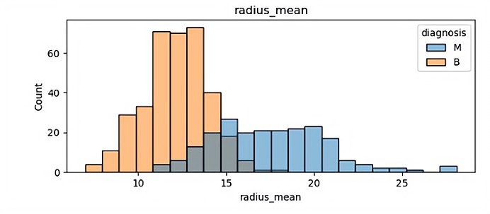
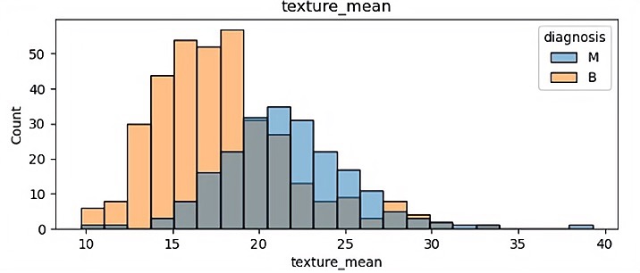
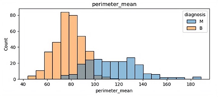
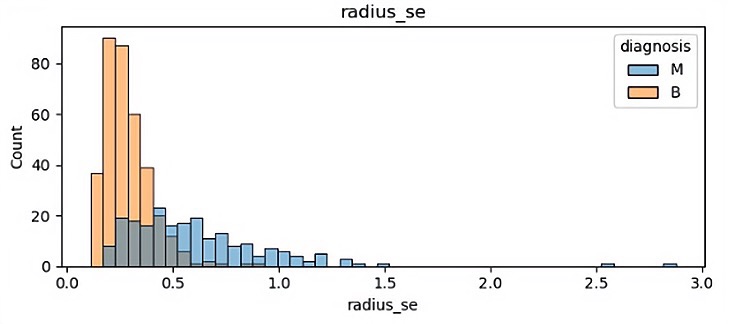
There are 32 different features so finally it has 32 different visualization results. In this paper, because of the space, some of the visualization results is been shown which are showed in Figure 1.
(a)
(b)
(c)
(d)
Figure 1. Visualization in the datasets.
In those pictures it can be seen that different features have a significant impact on malignant tumors and benign tumors. Benign tumors are usually smaller than malignant tumors, and they are widely separated. It will help the author classify in the future.
2.2. Data pre-processing
In order to classify the data easier, some attribute columns are been removed which are not useful for classification, for example: ID. For the rest of the columns, correlation matrix is been used to determine the correlation between features. From the correlation matrix, it can determine which features have a small impact on the benign and malignant aspects of tumors, which can directly ignore these features, which is also convenient to use random forests to extract the main features later. (correlation matrix will show in result part).
2.3. Modeling
In this paper, Random forest gain training set - bootstrap aggregation method(RF) is been used firstly to figure out 10 most important features that impact the benign and malignant tumors. Secondly, a SVM model is been trained based on these features for predicting the breast cancer, lastly, it is necessary to compare the model with three different machine learning methods including SVM, random forest, and PCA-SVM. The implementations are all based on Python3.
2.3.1. Support Vector Machine (SVM). An example of a supervised learning method used for classification and regression analysis is the support vector machine (SVM). Finding a hyperplane in a high-dimensional space that divides various classes of data points is the objective of an SVM. The distance between the hyperplane and the closest data points from each class is determined in a way that maximizes the margin between the two classes.
In addition to classification, SVM can also be used for regression analysis by predicting the value of a continuous variable rather than a categorical label. This is accomplished by finding a hyperplane that best fits the data while minimizing the error between the predicted values and the actual values.
2.3.2. Random forest: features selection. Random forest is a machine learning algorithm based on decision trees. It can be used for feature selection by calculating the importance of each feature. The basic idea of random forest is to build numbers of decision trees on random subsets of the training data and random subsets of the features, and then combine their predictions.
Random forest algorithm first uses the bootstrap aggregation method to gain training sets. A decision tree is built for each training set. When sampling using bootstrap, one sample is selected randomly from the original set (N samples) with replacement. One training set is generated by repeating this step N times. The probability that a single sample will be selected in N times of sampling is:
\( P=1-{(1-\frac{1}{N})^{N}} \) (1)
When n goes to in infinity:
\( 1-{(1-\frac{1}{N})^{N}}≈1-\frac{1}{e}≈0.632 \) (2)
This indicates that approximately 63.2% of the sample data is selected as the training set to participate in the modeling each time. Therefore, about 36.8% of the training data is wasted and do not participate in the model training. These data are called out-of-bag data (Out of Bag, OOB).
Suppose \( G_{n}^{-}({x_{n}}) \) to be the decision tree that OOB only concludes \( {x_{n}} \) . The number of decision trees of a random forest model is N. Then the out-of-bag error \( {r_{1}} \) is:
\( {r_{1}}=\frac{1}{N}\sum _{n=1}^{N}err({y_{n}}, G_{n}^{-}({x_{n}})) \) (3)
Let \( {r_{2}} \) be the error of the recorded random rearrangement OOB samples. The importance I for feature \( {x_{n}} \) is:
\( I({x_{n}})=\frac{1}{N}\sum _{i=1}^{N}({r_{1}}-{r_{2}}) \) (4)
After calculating the importance for each feature, sort the importance score and select the top 10 features for training SVM models.
In experiment, there are 16 decision trees in the random forest (n_estimator = 16 is gained by GridSearchCV). Based on the importance score, 10 most important features are been chosen for SVM prediction.
2.4. Evaluation
2.4.1. Confusion matrix. Confusion matrix can clearly show the results of the study. It shows confused predictive results. It can not only help to find the errors, but also display the types of errors. At the same time, other high-level classification indicators can be easily calculated from the confusion matrix.
2.4.2. Accuracy.Model accuracy refers to how well a machine learning model can predict the correct output for a giveninput. It is usually represented as a percentage or decimal value, where a higher value indicates better accuracy. Formula (5) is used to calculate the accuracy.
 (5)
(5)
2.4.3. Precision. The proportion of correctly predicted values to all actually correct values. In this study, it represents the ratio of cases where the model correctly predicts malignant tumors to all cases of actual malignant tumors. Formula (6) is used to calculate the precision.
 (6)
(6)
2.4.4. Recall. Recall refers to the ratio of the number of positive samples correctly identified by the model to the actual number of positive samples. In other words, Recall measures the proportion of models correctly identified in all actual positive samples, formula (7) is used to calculate the recall.
 (7)
(7)
3. Result
3.1. Result in data processing
Assuming that different eigenvalues are independent of each other, it can be seen from Figure 2 that 10 eigenvalues have strong correlation, 6 eigenvalues have strong correlation, 9 eigenvalues have weak correlation, and 5 eigenvalues have no correlation. This can lead to the conclusion that when extracting main features, it is unnecessary to consider features that have no correlation and weak correlation.
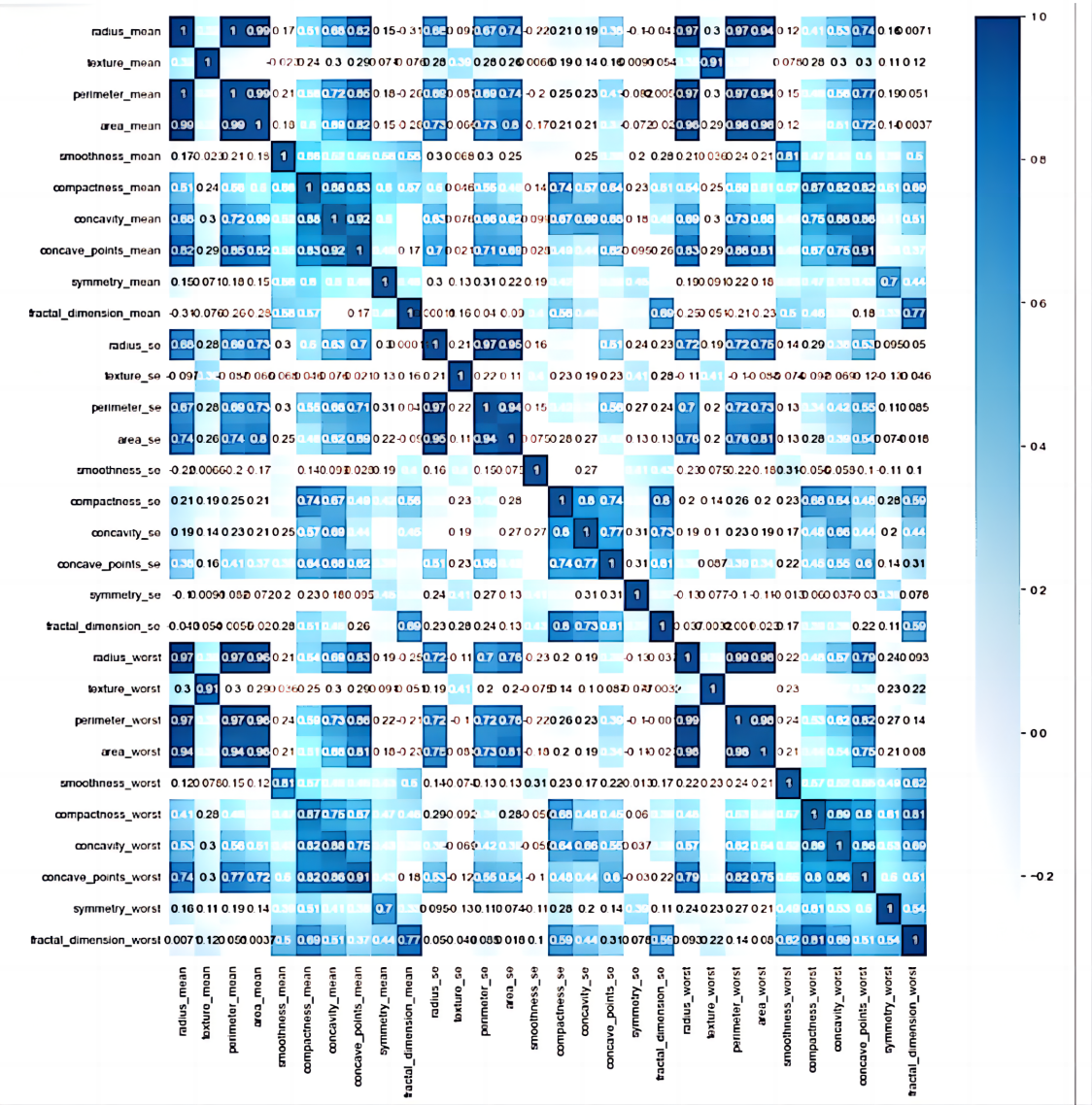
Figure 2. Datasets correlation heat map.
3.2. Result in main features extracting
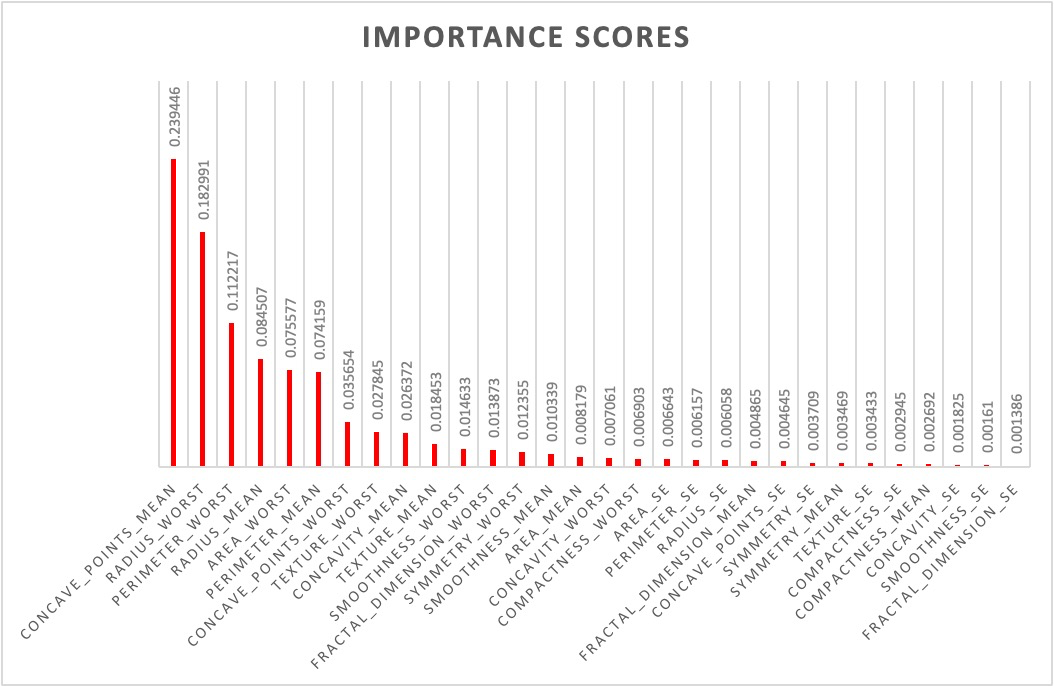
Figure 3. Importance scores of each features.
It can be seen in Figure 3 that different features have different importance scores, it is useful to choose the first 10 important features. They are listed in Table 2.
Table 2. The first 10 important features.
Feature | Importance scores |
concave_points_mean | 0.239446 |
radius_worst | 0.182991 |
perimeter_worst | 0.112217 |
radius_mean | 0.084507 |
area_worst | 0.075577 |
perimeter_mean | 0.074159 |
concave_points_worst | 0.035654 |
texture_worst | 0.027845 |
concavity_mean | 0.026372 |
texture_mean | 0.018453 |
3.3. Classification results
The result of the model compares with other three models is shown in Figure 4. Figure 4 shows classification results of RF-SVM, RF, SVM and PCA-SVM methods. For accuracy, it observed that RF has the highest accuracy (0.97), but for the precision it observed that SVM has the highest precision(0.98).
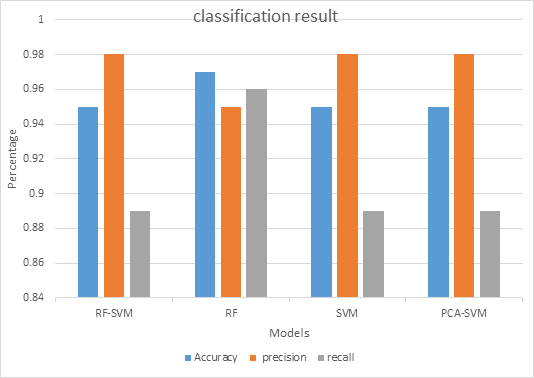
Figure 4. The classification performance of models.
3.4. Result comparison
The confusion matrix results of the SVM, random forest and PCA-SVM are demonstrated displayed in Figure 5, 6 and 7. From the confusion matrix it observed that SVM predict 86 are class 0 and 52 are class 1 and there are 5 predict wrong. That means it has a high accuracy(0.95) but it has a lower precision. As for PCA-SVM it has the same performance and RF has the highest recall(0.96), there are 88 are class 0 and 48 are class 1.
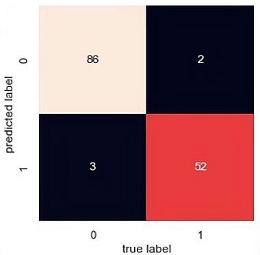
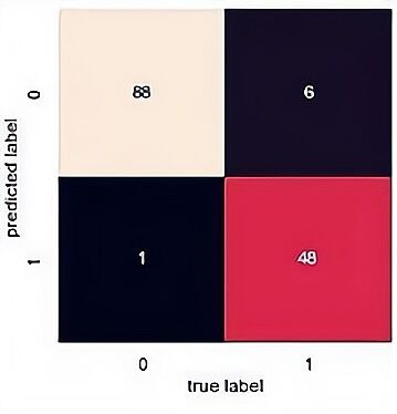

Figure 7. PCA-SVM.
4. Discussion
The performance of the three models met expectations. It is worth noting that the performance of the PCA-SVM has a higher accuracy. From the result part it shows that although Random Forest has high accuracy but the precision is low. From the primitive study on compressive strength of concrete[9], it can be seen that RF has eliminating the impact of some unimportant redundancies effectively, but as the features goes more and more, the precision goes lower and lower. In order to get higher precision an optimal combination must be found to meet the need. As for RF-SVM, it has higher precision more like SVM, from [10] it can observe that when build a SVM model it has to introduce a kernel function to transform the low dimensional nonlinear problem into a high-dimensional linear problem. Optimizing parameters to find the highest precision to be the input, as for RF it’s just a method to do the variable culling, to make sure SVM will preform better, it make no sense to the precision.
5. Conclusion
It observed that the model RF-SVM achieve 95% high accuracy. If compare RF-SVM with SVM, it can be seen that they gain the same accuracy, precision and recall. This indicates that some features are useless in predicting the tumors. If compare RF-SVM with PCA-SVM: both have dimension reduction step. The accuracy, precision and recall are similar because they both use SVM. However, RF-SVM complete the training in a much shorter time, which is more efficient. If compare RF-SVM with RF: although RF has higher accuracy, precision and recall, the training time of RF is three times as long as RF-SVM. Overall, RF-SVM can achieve high accuracy (95%). There also needs more data to train and in the future, it is still really important working on optimizing the model, in the future, the author wishes the accuracy will be higher than this one and the advice on improving the model from readers is welcomed.