Which network is stronger? Le Net, Alex Net and VGG on image classification

1. Introduction

Image classification is a method that assigns a label to the given image to identify the category the image belongs. The metric is to differentiate the image from each other after being processed like the intensity of pixels, and edge detections. Image classification has been proposed for a long time and it is in high demand in society such as in the medical imaging area, satellite imaging, etc. Moreover, image classification has been popular in machine learning, many classic deep learning neural networks were born to facilitate the image classification work.

The methodology on it has been developed through the decades. In traditional machine learning, the image classification needs to experience feature extraction, and feature selection, and then the feature vectors are put forward into the suitable classifiers to complete the feature classification. SIFT algorithm is also proven to be effective in image classification tasks in the beginning of this century [1]. In recent years, with the development of deep learning neural networks, the image classification task is also proven to work well on the convolutional neural network. The research on CNN is continuing and there is great potential to improve CNN's performance on image classification. The LeNet is a classic CNN network proposed by Yann LeCun in 1989 which was designed on the dataset MNIST to do the classification task, it is a simple framework and has a relatively small number of parameters, although it is relatively old, it still has widely used and give much inspiration to the other network structures. AlexNet was proposed by Alex Krizhevsky and is also a classic neural network, it has a similarity with LeNet while it is more complex, and it is thought to be a milestone in the deep learning area. VGG is thought to be the next step of AlexNet. The three convolutional neural networks are widely used and referenced in nowadays research.

This paper will focus on the cases that them to be applied to image classification, with the analysis of the performance, strength, and weakness, the article will give the appliable scenario of the three classic convolutional neural networks.

2. Method

Being considered one of the most powerful tools in Artificial Intelligence [2], the convolutional neural network is proven effective and strong to process a large amount of data. Inspired by the human brain, the convolutional neural network was designed to process multi-dimensional data [3], the data will be processed and passed to the next neuron in the network. With the difference from the regular neural network, the layers in the convolutional neural network are three-dimensional: width, height, and depth. And the neuron in the convolutional neuron network will be connected with a part of the previous layer instead of fully connected. besides the input layer and output layer, the CNN architecture has multiple convolutional layers and pooling layers. The convolutional layer is for the convolution and the pooling layer is used for local averaging or maximizing, usually the width and the height of the convolutional layer while the depth will be increased. LeNet, AlexNet and VGG are classic convolutional neural networks and they are developed in lots of research and project, they share some similarities but the structure made them different, and perform differently.

2.1. LeNet-5

LeNet is proposed by LeCun in 1998 [4]. It was designed for the database MNIST [5]. The structure of the LeNet-5 is relatively simple(as shown in Figure 1).

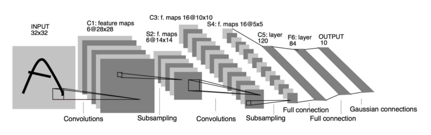
A size 28 by 28 image is passed as input of LeNet-5, followed by two layers. each layer consists of one convolutional layer and one pooling layer. The dimension of the width of height gets smaller mainly because of the subsampling and the number of channels(depth) gets larger as more filter will be applied as the network go deeper. After the process of the two layers of convolution, the network is flattened into one dimension and becomes a fully connectional layer. With 120 neurons reduced to 84 then 10, the network will give a layer with 10 values as output.

2.2. AlexNet

AlexNet was designed by Alex Krizhevsky [6] in the competition of ImageNet, reaching an amazing 15.3% error rate [3]. The art of AlexNet lies in the depth, it is much deeper compared with LeNet-5. While the key structure of it is similar to LeNet-5, in which the convolutional layer is followed by a pooling layer multiple times and then flattened to one-dimensional and become a fully connected layer (shown in Figure 2).

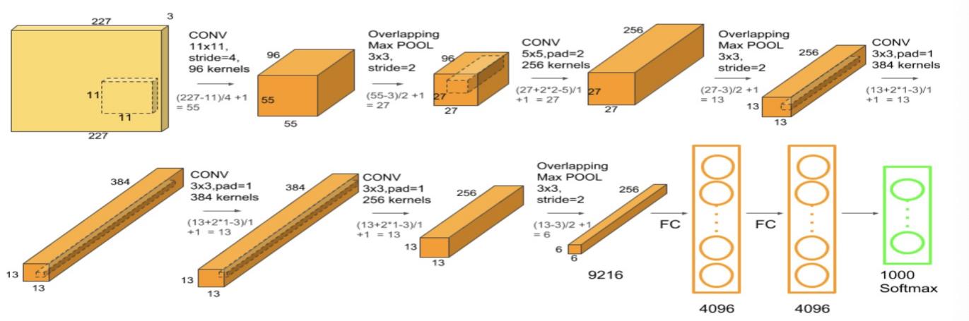
The input image of AlexNet is larger than LeNet which is 227 by 227 the depth is 3 as the input image is an RGB image it has three channels representing red, green, and blue. Then the input is passed to the convolutional layer, followed by the max-pooling layer. Before the last max-pooling layer, the same padding was applied three times. Then similar to the LeNet the network is flattened and becomes a fully connected network. The AlexNet is much deeper and larger than LeNet. There are 60 thousand parameters to be trained in LeNet while the number becomes 60 million in AlexNet. So AlexNet will be run on cuda or GPU.

2.3. VGG

VGG is proposed by K. Simonyan and A. Zisserman in 2014 [8]. It improved on AlexNet by using the 3 by 3 filter and doing the same padding, and then the network makes the max-pooling layer 2 by 2 with the stride of 2, which made the advantage of VGG that it simplify the architecture of the network (shown in Figure 3).

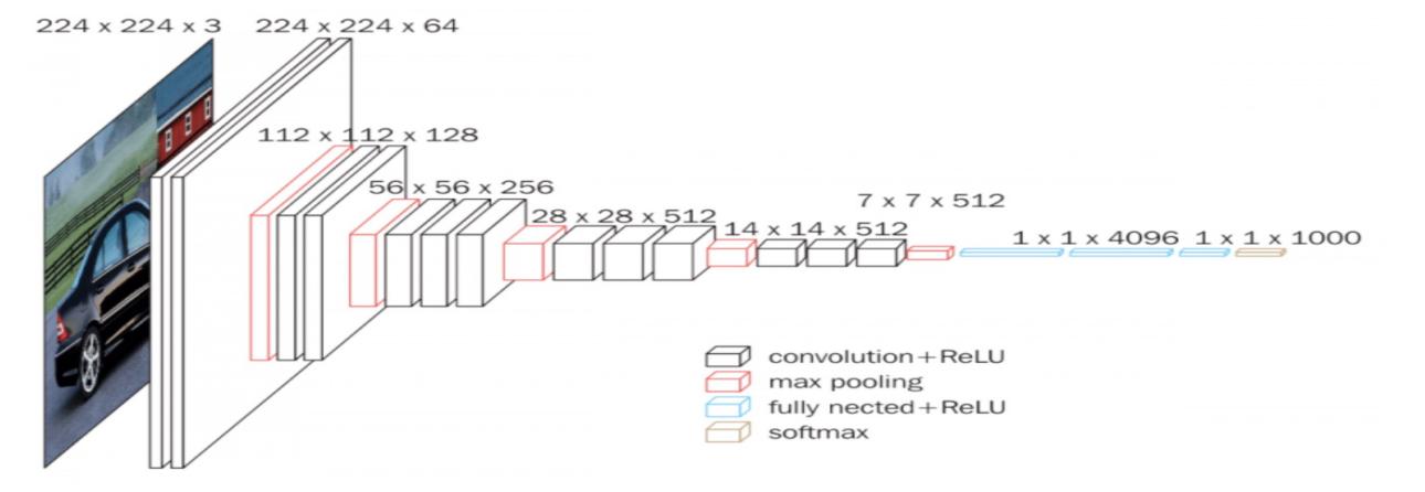
As Figure 3 shows, the architecture of VGG is uniform, which is a convolutional layer followed by a pooling layer and then enter the next convolutional layer. The width and height of the convolutional layers are halved while the depth is doubled until the depth reaches 512. It has over 138 million parameters which make it remarkably large by modern standards. So like AlexNet, the VGG is also run on CUDA or GPU by convention.

2.4. Loss Function

For the Loss function, the classic Cross-entropy loss function will be used. The formula is given below.

\( L=\frac{1}{N}\sum _{i}{L_{i}}=-\frac{1}{N}\sum _{i}\sum _{c=1}^{M}{y_{ic}}log{(p_{ic}})\ \ \ (1) \)

With M representing a category, y represents 0 or 1, if sample i belongs to c then y equals 1, otherwise, 0. p represents the probability that the sample i belongs to category c. The model is trained on the dataset which has multiple categories, where the cross-entropy loss is well-behaved in this experiment.

3. Experiment

The experiment will use CIFAR-10 to be the dataset. After being processed by the three networks and the classification task taking place, confusion matrix analysis will be the main metric to evaluate the performance of the three networks. The experiment runs on GPU as the parameters to be trained on AlexNet and VGG will be significantly large, normal CPU could not afford such a workload.

3.1. Database choose

The data in the image dataset used in the experiment should represent the feature well and the dataset should have enough images to train the model. Based on the criterion above, the CIFAR-10 is chosen to be the dataset in the experiment used to train and test the performance of the three neural networks. CIFAR-10 comes from Canadian Institute For Advanced Research. The dataset has t10 classes of images representing 10 categories, and each class has 6,000 images. CIFAR-10 is proven a well-performed database in the convolutional neural networks, it fits the three networks in the experiment well by doing the simple resize operation.

3.2. Data splitting and hyperparameter setting

According to the convention of data splitting, 1,0000 CIFAR-10 images are used for testing data and the remaining 5,0000 images are used for training data. The split is also what the CIFAR-10 dataset originally indicates. Concerning about the hyperparameter setting, the hyperparameter are tuned to set as the values below(shown in Table 1). The metrics of evaluation will mainly focus on accuracy, the first aim of the hyperparameter setting is to make the three networks perform their advantages, optimizing the performance to a small-scale decimal point and digging deeper of the three networks are not considered.

Table 1. Hyperparameter Setting.

3.3. Result and discussion

The result is shown in the table below（Table 2）, all the measurements were taken on the testing dataset. The accuracy is measured overall samples from 10 classes, while the precision, recall, and F1 score of the ten different classes were measured separately and the data shown below are the average value. It is easy to observe that VGG has the most outstanding performance on the accuracy, which achieved the value 0.93. The AlexNet comes from the next which achieved an accuracy 0.76 while the LeNet achieved 0.53. Intuitively speaking, the VGG has the deepest structure and has the most parameters trained, then AlexNet has the second most parameters in the network while LeNet is the simplest among the three networks, which explains the accuracy to some extent.

Table 2. Evaluation of Three Networks.

LeNet was designed to classify the dataset MNIST and the dataset consists of the digit number from zero to nine and the images were in black and white, the research has shown that LeNet performs outstandingly on MNIST and achieved over 0.9 accuracy [10]. However, the images in CIFAR-10 are much more complex, the images have three color channels for Red, Blue, and Green and the contents and features represent more than MNIST. The structure of LeNet is relatively simple among the three networks and it is not as deep as the other two, which makes it perform not so well compared to AlexNet and VGG. One thing to note is that because of the structural property of LeNet, the training time is the shortest and it only needs about 1 minute time for training.

About the AlexNet, the overall metrics are better than LeNet. The accuracy is 0.76 which is acceptable. However, if we go deeper into the measurement of AlexNet, we can see that for most categories like airplane, truck, and ship. The AlexNet can classify them well and achieve over 0.8 accuracy. But when comes to cats, deer and dogs the accuracy suddenly dropped to around 0.6(shown in Table 3 below), and this is the reason that the accuracy of AlexNet is not as good as VGG. The reason is that the three categories are animals and share some common features. The resized images are vague so the features are not well-represented. About the transportations like airplanes, trucks and ships, they clearly differ from each other and the features point to them directly. AlexNet performs well comprehensively, the training time of it is around 5 minutes from which the fact can be denoted that the time AlexNet taken is much shorter than VGG.

Table 3. Accuracy on each class of three networks.

Although VGG takes the most execution time, it achieves the highest accuracy, the measurement indicates that VGG performs best in the three networks. Compared with the analysis of the LeNet above, VGG has the most parameters trained, over 130 million parameters. The results show that it classifies all the classes in CIFAR-10 well, with most classes achieving over 0.9 accuracy, the performance on accuracy is good and does not have much space to increase, a feasible improvement can be data augmentation[5]. The VGG net has another issue which worth a discussion in the experiment, as it has a large number of parameters in training, the running time is relatively too long and it took too much space of RAM, which means some device may not afford it such workload. The experiment of VGG was first taken on the GPU of the device Macbook 2021, then the core ran out because the RAM could not afford the experiment, then the experiment was taken place on Google Colab Cloud Server and successfully executed. Even though the execution time takes 30 minutes which is much longer than VGG and LeNet.

4. Discussion

This research found that the three classic convolutional networks have their advantages and disadvantages which are decided by their inner structures.

The LeNet has a relatively simple structure among the three networks which made it runs within the shortest time. It performs well on some datasets which did not represent too many features like MNIST. However, when it works on some more complex datasets like the CIFAR-10 in this experiment, the result shows that accuracy of LeNet is not as good as the other two networks, which may not meet the criterion of industry. Considering that LeNet is the oldest network among the three, it came earlier many years before AlexNet and VGG, the networks that came later gained a lot of inspiration from LeNet, and the performance it does on CIFAR-10 is still commendable.

About the VGG it performs best in the accuracy aspect. The complex structure of VGG extracts and trains the features well on CIFAR-10. The accuracy over 0.9 does not have too much space for improvement, although some more experiments can be held to optimize the performance of VGG like data augmentation, the accuracy that comes out from the experiment is remarkable. However, the large workload is a disadvantage of VGG, this is a simple tradeoff that the complex structure gives the network outstanding performance on accuracy but sacrifices the running time. Sometimes the experiment may take hours and the RAM space may run out.

Comprehensive speaking, the AlexNet is thought to be the best network by the author in this experiment. Although it has lower accuracy compared with VGG, it has a much shorter execution time, the accuracy around 0.8 is acceptable and it can be improved in many ways which would not sacrifice to much execution time. Some practical operations for improvement can be inserting another convolutional layer after the original 5 convolutional layers.

5. Conclusion

This paper mainly illustrated the structure of the three classic convolutional neural networks which are LeNet, AlexNet, and VGG. The research on how they work on the image classification task on the CIFAR-10 dataset is also illustrated. The three networks are widely used in many research and the modern networks gained a lot of inspirations from them. This research gave a quantifiable analysis of the three networks and demonstrated their advantages and disadvantages. some facilitations may be applied to combing the strength of the three networks to develop a model with a considerable performance on accuracy and execution time.