Comparison among baseband codes based on MATLAB

1. Introduction

Digital baseband signal is the original signal that is yet not be modulated. There are various kinds of code patterns and they can be catalogued approximately as NRZ (no return to zero), RZ (return to zero), unipolar, bipolar et cetera. Different waveforms have their unique characteristics in several respects, affecting the qualities of the whole communication system, thus there are different coding patterns applicated in various fields. Exploring these waveforms’ advantages and disadvantages are helpful to understand the usage of code patterns in various situations, satisfying prerequisite for inventing new code formats. The research will mainly look into 3 aspects. First and foremost, the capability of resisting error bits will be looked into between unipolar and bipolar signals. Researchers have been figuring out ways of error control like error-correcting codes, and cyclic codes are used to be the most promising codes, especially the burst-error-correcting codes are the most attractive and fascinating according to W.W.Peterson [1]. What is more, algorithms of coding and decoding are also being utilized to ensure high ability of the noise immunity. Martynov and his co-workers presents analysis and assessment of the implementation of digital information channels(DIC) based on code signal feature (CSF) [2]. Ensuring a high ability to resist noise resulted from rising requirements of quality in communication is essential. In the second aspect, the paper will demonstrate comparison of channel capacity based on Shannon formula. Channel capacity is a significant element promising the reliability of communication. As communication technology develops, methods of propagating information become ample. Investigations about channel capacity take place in different methods of communication. In wireless communication, Farzamnia and his team studied channel capacity enhancement using hybrid algorithm [3]. In another field as optical communication, there are also similar researches. Optical communication uses laser to communicate, loading information on many characteristics of lasers in order to transmit reliable information. Optical communication owns great advantages, such as extremely fast speed, outstanding channel capacity, hard to be stolen, high resistance towards electronic disturbs. While in this field, Essiambre works with his colleagues, describing a method to estimate the limits of channel capacity in optical communication based on information theory [4]. Channel capacity is an essential element of promising reliable communication that worth exploring. Furthermore, the performance of different codes in frequency domain will be illustrated. Signal’s performance in frequency domain affects their overall advantages and disadvantages when promulgating. Furthermore, characteristics of signals in frequency domain can be useful generating new signals, this is proved in Mirchandani works. Mirchandani used to generate discrete-time analytic signals using frequency domain method [5]. Lastly, the thesis will illustrate part of the popular coding patterns used nowadays which own characteristics discussed above. The codes generated are Manchester, AMI and CMI. They are all popular and being applicated in different fields and situations but owning completely different features. All these four aspects’ images and modulations mentioned will be demonstrated based on MATLAB, a powerful software that is often used to do research on academic fields. The thesis will make comparisons separately on levels of noise resistance, channel capacity and performance in frequency domain, and lastly generate some particular coding patterns using MATLAB. This thesis will be based on fundamental knowledge, representing knowing results with more figurative illustrations, helping better understanding the meaning of the born of different code formats using figurative illustrations and analysis which are educational meaningful. By doing so our thoughts can better anew.

2. Comparison between unipolar signal and bipolar signal in capability resisting noise

Most characteristics of unipolar and bipolar signals are similar. The difference appears when logic ‘0’ being promulgated. In unipolar waveforms, logic ‘0’’s amplitude is 0, while in bipolar signals, the amplitude becomes ‘-1’, making the electrical waveforms have both positive and negative values, which also make the value of peak-to-peak amplitude different. Fig.1 showing below is generated on MATLAB.

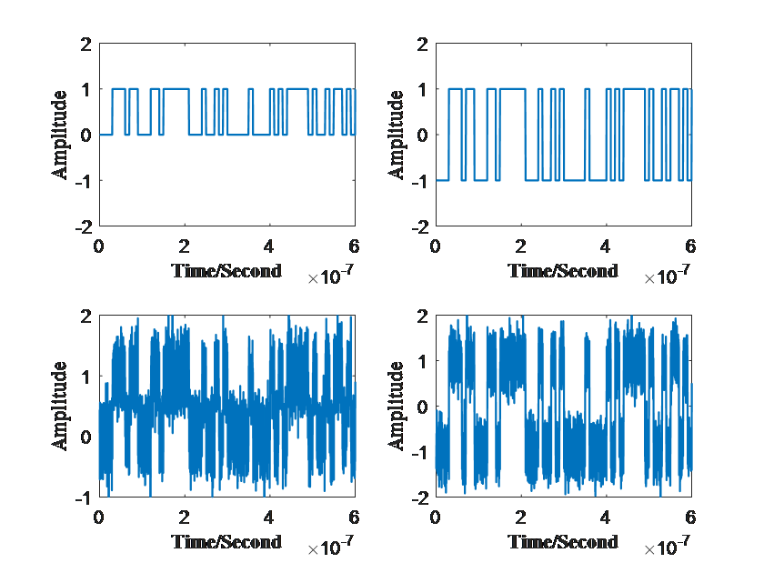
It is assumed that bigger peak-to-peak values render it more capable of resisting the effects of noise. The assumption is reasonable since larger peak-to-peak value allows the existence of greater noise. For instance, if there is a noise pulse owning values slightly more than 0.5(positive) and the middle of peak-to-peak value as the threshold is set, when this occurs to unipolar signals, the ‘0’ bits will be checked as ‘1’ wrongly. Meantime, if the same situation happened to bipolar signals, ‘0’ bits have ‘-1’ level and influences of noise will not harm the accuracy of bits transported. Evidence of it will be provided using MATLAB.

First and foremost a bitstream modelling digital baseband signal will be generated randomly using function ‘randi’ and it contains 5000 bits in total. In MATLAB, ‘N’ is set to represent the quantity of bits and ‘data’ the vector presenting the original information.

After this unipolar signals and bipolar signals can be generated. It is relatively easy to generate unipolar signal first so that the bipolar ones are conveniently generated. Assuming that ‘data’ is the unipolar signal, then ‘data2’ representing bipolar bitstreams can be calculated by twice times ‘data’s value minus 1. In this case, ‘1’ bits are still ‘1’ while ‘0’ bits become ‘-1’ so that bipolar signals are born.

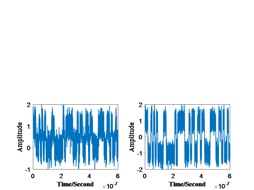
After the generations of the two different waveforms, then additive Gaussian noise is added to it, so that the process of transmitting could be modelled. At this step function provided in MATLAB called ‘awgn’ can be utilized. Inputs are signal-to-noise ratio and bitstreams needed handled, then the original signal with additive white Gaussian noise can be got. In this thesis, signal-to-noise ratio is set 10. With codes discussed above, the signals with additive Gaussian noise generated are in Fig.2 as follows:

The next essential step is to simulate the function at the receiver side. Sample signal is generated sampling the value of waveforms at the middle of every bit’s period. Then comparison is made between received bitstreams and the original bitstreams so that could error bits, can be marked and counted calculating the BER rate lastly. Signal-to-noise ratio changes from 1 to 20 and applicated the procedure discussed above at each SNR value. Furthermore, in order to demonstrate the accuracy of the process, the procedure is run 10 times at every signal-to-noise ratio spot, drawing curves attached with error bars. In order to do accomplish all these aspects, fundamental elements of the loops need to be set. ‘m’ is an essential variable to document sequence when running the procedure. Then various of matrixes are created. First there comes ‘rep1’ and ‘rep2’ to calculate BER rates through every single time of testing. Moreover 8 vectors replete with zeros are created. ‘count1’ and ‘count2’ are vectors recording the quantity of error bits. With two vectors discussed formerly, ‘ber1’ and ‘ber2’ can be set to document the means of BER rates through ten times at every signal-to-noise value. ‘ber1errorup’ and ‘ber2errorup’ are created in order to calculate the upper bound of error bars. At the opposite side, ‘ber1errordown’ and ‘ber2errordown’ are set to gain the minimum value of error bars.

All variables above are set to facilitates calculation and convenience of MATLAB codes’ running. Loops thus can be run with these elementary variables. The most outside loop is for signal-to-noise ratio ranging from 1 to 20, while the loop inside varies from 1 to 10 so that BER rates’ values at all signal-to-noise ratio point can be gained ten times ensuring the accuracy. Each time when the smaller loop is finished meaning BER rates at one signal-to-ratio point is gained, mean of those ten values will be calculated and their ranges will be got to acquire information about error bars, and the flag ‘m’ mentioned formerly must plus 1. During each time of calculating BER rate, original signal will be mixed with additive white Gaussian noise using ‘awgn’ function to calculate directly. Then function of the receivers will be modulated to get received bitstreams. Sequentially received bits are compared with original ones to count the number of error bits so that BER rates are acquired. Repeatedly running this procedure through elaborated loops can help gain sufficient results to draw curves with error bars attached.

Applicating ideology above is able to generate the image with error bars below in Fig.3.

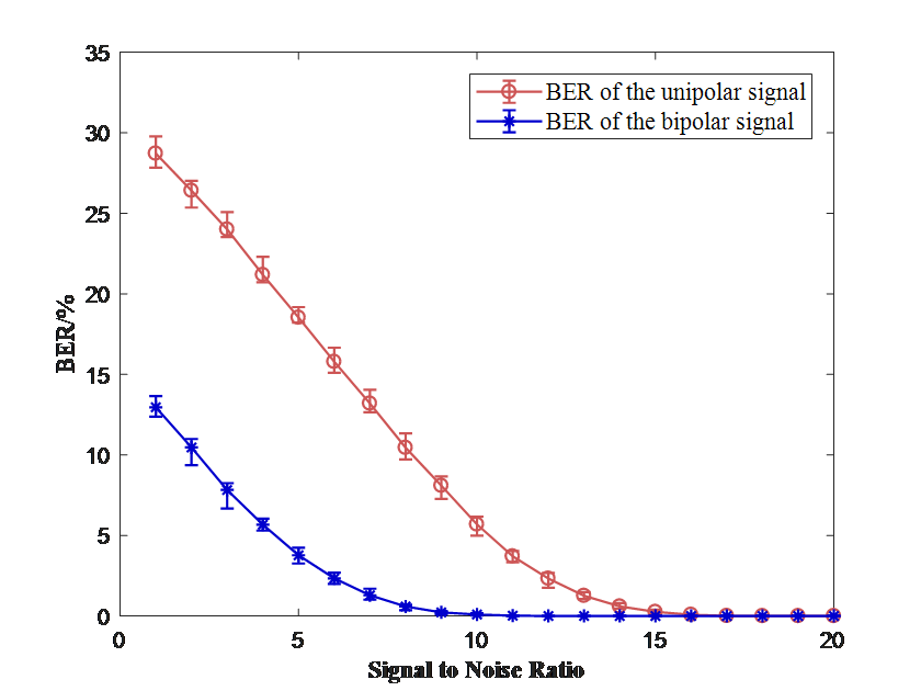
In Fig.3, it is obvious that when SNR rate increase, BER rate of both unipolar and bipolar signal decrease. During this process, BER rate of bipolar signals is always lower than unipolar signal, which authenticate the speculation mentioned above. Furthermore, error bars on all points are different but generally short, meaning that the accuracy of the data is promised.

Besides, during the research, it is suspected that the quantity of bits being promulgated can also have effects on BER rate calculated. Thus, the number of bits vary from 50 to 4000 and calculate log of BER (base 10). To start the procedure, rudimentary variables and vectors needed to be firstly set up. Variable ‘m’ functions as a flag just as the last part of codes. Sequentially 4 vectors replete with zeros are constructed. ‘ber1’ and ‘ber2’ function as documents gathering information about the value of BER rates. These calculations require vectors ‘count1’ and ‘count2’ to count the quantity of error bits. After elementary constructions, loop ‘N’ is set ranging from 50 to 4000. ‘N’ represents the number of bits being promulgated. Within the loop, the very first step is to create unipolar data and bipolar data as usual. Then just as what the later procedure run, white Gaussian noise is added and receivers’ functions are modelled so as to acquire BER rates.

These codes above can help readers produce these outputs again and also make sure that all the logical details are acceptable and considered carefully. The curves generated are demonstrated below in Fig.4.

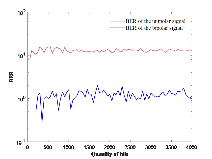
Initially, quantity of bits being transmitted is only around 500 to 1000. It is found that the fluctuation is relatively severe, meaning that the results are inaccurate. As the number of bits enlarged, the fluctuation of BER rate becomes gentle. This pattern shows that more bits generated is significant to the authenticity of experiments depicted in this paper.

3. Comparison between NRZ and RZ signal in channel capacity

Non-return-to-zero and return-to-zero waveforms differ from the other when comes to the middle of bits’ periods, which also render them have different channel capacities. Based on Shannon formula, bandwidth and signal-to-noise ratio are changed separately, illustrating the fluctuation of channel capacity. In Fig.5, curves show that when SNR ratio rises, both NRZ and signals’ channel capacities increase as well. RZ signal’s channel capacity, however, remains greater than NRZ’s. The causation is the difference of bandwidth in frequency domain discussed in the next section.

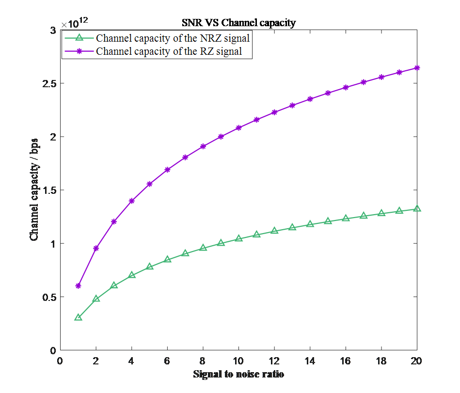
Figure 5. NRZ signal and RZ signal’s channel capacity when signal-to-noise ratio increase.

(Photo credit: Original)

4. Comparison among the matched waveforms in frequency domain

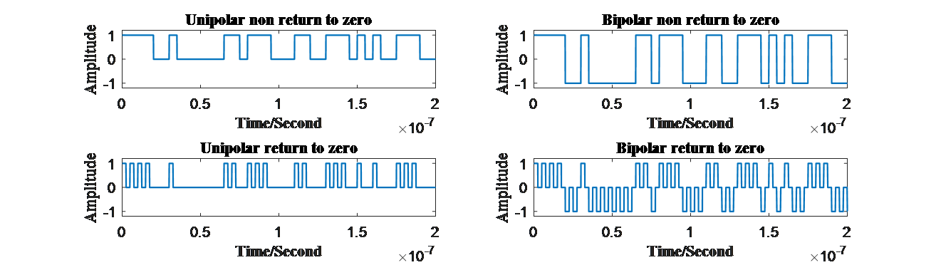
If these different characteristics are matched, 4 different waveforms will appear: unipolar non return to zero, bipolar non return to zero, unipolar return to zero, bipolar return to zero. The waveforms are as follows demonstrated in Fig.6.

Utilizing MATLAB these waveforms can be transformed from time domain to frequency domain, where some features are able to be observed more clearly just as shown in Fig.7.

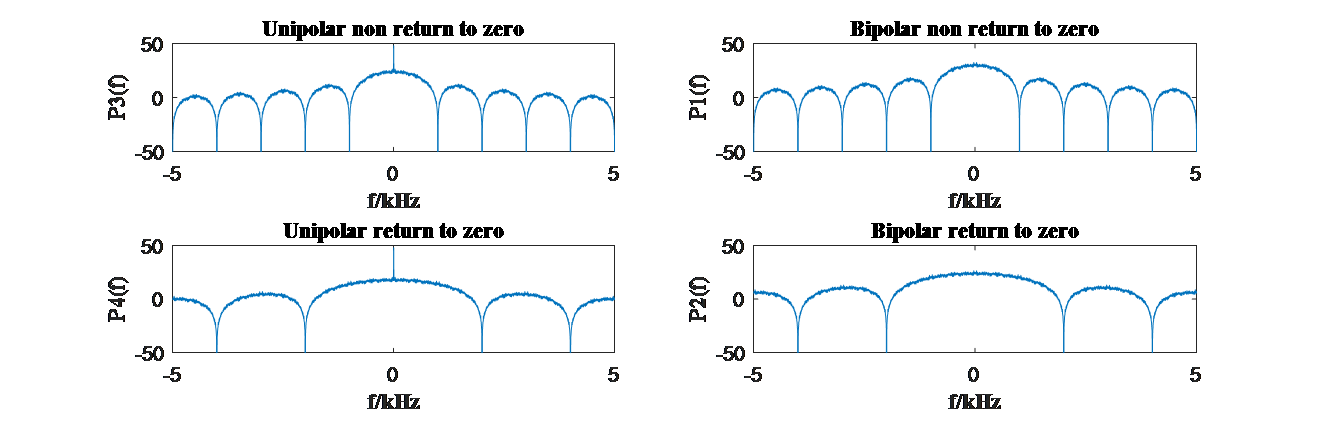
The variety lies mainly on bandwidth and whether there are pulses attached. Apparently, bandwidths of RZ signals are relatively larger than NRZ signals’, rendering RZ signals own greater channel capacities when SNR ratio is the same. This lateral has its disadvantage as well. Larger bandwidth also occupies more resource and has a negative effect on spectral efficiency, an essential assessment standard describing communication systems.

Besides the difference in bandwidth, only unipolar signals have pulses while bipolar ones do not. These pulses are able to facilitate the works of timing at receiver sides.

5. Generation of common baseband waveform (Manchester, AMI, CMI code)

Finished comparing these various kinds of codes, common codes used nowadays is generate. All of them are the applications and improvement of the waveforms discussed above. To generate these codes, an original signal is firstly needed to be produced in order to produce different coding patterns more conveniently just discussed at the very beginning parts using function ‘randi’ offered by MATLAB itself. Furthermore, in order to demonstrate bitstreams on figures, original bits are supposed to multiply vectors filled with ones to generate vector ‘datao’ so that original bits can be illustrated on time axis more conveniently.Among the codes above, ‘datao’ represents original bit streams.

Manchester code is one of the most popular codes. It brings lots of advantages especially for high-speed burst mode transmission, and its ability of simple clock recovery and level recovery enable its high resistance towards signal intensity fluctuation [6]. Moreover, Manchester code also reduces the existence of low frequency components [7], helping researchers creating more applications. The coding pattern is that turn “0” to “01” and change “1” into “10”. Manchester codes are usually transmitted in bipolar NRZ waveform. The methodology of generating it with MATLAB is simple. First and foremost, a 0,1 bitstream will be created randomly to model the sending information. Then a circulation will be implemented and ran until all the original bits are dealt with. In each loop a “0” or “1” will be changed into “01” or “10”. First and foremost, vector ‘mac’ is set standing for Manchester bits. Then loops running from 1 to ‘N’ presenting number of bits is constructed. Faced with each original bits, if it is ‘1’, then ‘1’ and ‘-1’ will be wrote into ‘mac’ sequentially. When it comes to ‘0’, ‘-1’ and ‘1’ are wrote into ‘mac’.

AMI code, known as Alternative Mark Inversion, lets electrical level 0 represents digit “0”, and change the polarity of electrical level 1 every time coming to another digit “1”. Because of the changing polarities of levels, AMI code is able to check error bits. Therefore, AMI code is usually focused on error detection schemes [8]. First and foremost, variable ‘flag’ needs to be set to count the times facing ‘1’ and vector ‘ami’ is constructed to fill in AMI bits. Each time when comes to ‘0’, ‘0’ will be filled into ‘ami’ without changes. However, when comes to ‘1’, whether the number of ‘1’ is odd or even has to be decided so that whether to write ‘-1’ or ‘+1’ can be decided.

The last pattern shown is the CMI code. Similar to AMI code, the electrical level presenting “0” remains unchanged as “01”, and the other transformed by digit “1” changed from “11” to “00 ” or the opposite each time a new digit “1” appears. The difference is that CMI code will not have more than three successive bits, which does great help examining error bits.

Among the codes, ‘cmi’ represents the CMI codes produced. When generating these different codes in MATLAB, the most essential aspect needed to be paid attention is the time axis, especially when changing objects from NRZ codes and RZ codes. Careless manipulation will cause errors to a great extent.

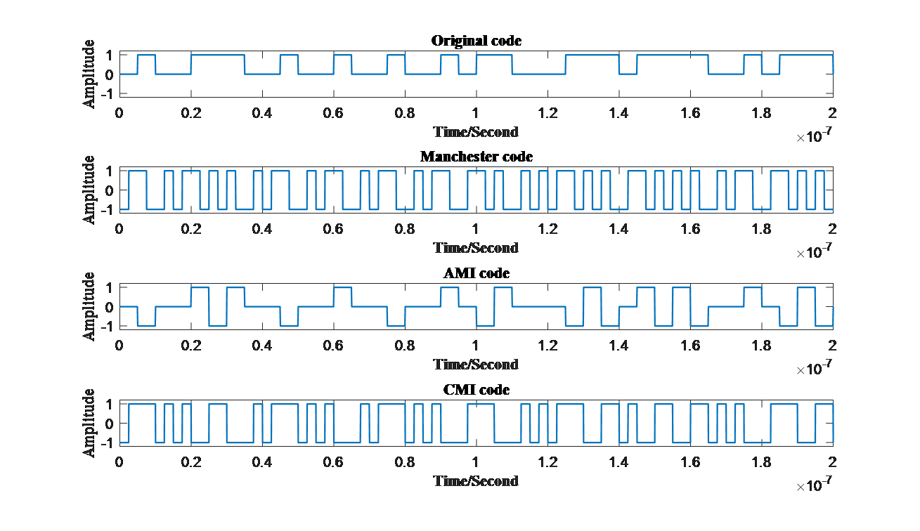
Similar to Manchester code, CMI code also has great capabilities recovering clocks, which can be applied into realistic products [9]-[10]. All different kinds of codes generated are demonstrated below in Fig.8 .

6. Conclusion

To sum up, bipolar signals do own greater ability when resisting noise compared to unipolar signals. Moreover, the accuracy of the result is promised since the experiment generate 5000 bits to debate fluctuation among different times of experiment. As for difference between RZ and NRZ waveforms, RZ waveforms is proved to have greater channel capacities, but this advantage has its cost. It is clear that RZ signals have bigger bandwidth but this may harm spectral efficiency. Unipolar waveforms have their own advantages as well, owning pulses helping timing. When the different elements discussed above are matched, different codes is generated using corresponding patterns. Each of them contains advantages depended on their shapes.