Predicting implicit operators among solutions for certain differential equations systems with DeepONets

1. Introduction

The essential governing equations of most physics and chemistry models in many engineering areas are differential equations, such as mechanical vibration or structural dynamics, heat transfer, and fluid mechanics [1]. There are two main methods of solving a multivariate differential equation system nowadays: the numerical method and the machine learning method. However, the high stiffness of a multivariate differential equation system will prevent the traditional numerical methods to solve it fast and accurately [2]. The neural network method has been developed for 20 years [3], and its application in modeling physics problems have also been explored with various neural network architectures such as deep neural networks, convolutional neural networks, recurrent neural networks, and physics-informed neural networks. It’s been a growing appreciation of the employment of machine learning in approximating the physics governing functions, which are usually differential equations since neural networks have the ability to fast and accurately model lots of complex problems hardly addressed by traditional numerical methods. Although the stiffness does not influence the machine learning methods in solving multivariate differential equations systems, there is still a limitation that it cannot be solved systematically like numerical methods. It’s hard for neural networks methods to take the small number of inputs (initial conditions) and generate a large number of outputs (functions which are essentially lots of discrete points) or it will considerably influence the quality of the model that the parameters in the model usually hardly converge [4].

Deep multiphysics and multiscale network (DeepM&Mnet) [5] is proposed to predict the coupled flow and finite rate chemistry behind a normal shock using a neural network approximation of operators [2]. It consists of a deep neural network and several other neural networks, Deep Operator Network (DeepONet) [6] which is used to predict both explicit and implicit operators such as antiderivatives, 1D Caputo fractional derivatives, 2D Riesz fractional Laplacian, nonlinear ODE, and PDE, etc, based on a less known fact that neural networks with one hidden layer can also accurately approximate any nonlinear continuous operator [7]. DeepM&Mnet successfully outputs several functions of densities of various chemistry compositions, temperature, and velocity given just small amounts of inputs which is the location information. The pre-trained DeepONets approximate the implicit relations among those outputs and assist to train the DNN in DeepM&Mnet.

In this paper, we use DeepONets as the building blocks to train an accurate model for certain multivariate differential equation systems. The object of the model is to generate solutions of a certain multivariate ODE and PDE system given any initial condition. We used DeepONets as building blocks to test and predict the implicit relations among solutions of the differential equation system for further construction of the framework. The relations were tested to be existing and well predicted by the DeepONets, which will be used later to build the frame of the network taking inputs of initial conditions and outputting solutions.

2. Method

The main idea of the proposed framework is to map an input which is the initial conditions of a certain differential equation system into outputs which are the solutions of it. DeepONets play the role of building blocks in the framework to predict the potential relationships among the solutions, that are used as the operators mapping solution of one variable into that of another. Then these building blocks will be later used to construct the proposed framework.

2.1. DeepONets

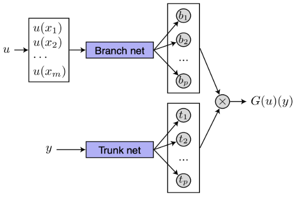
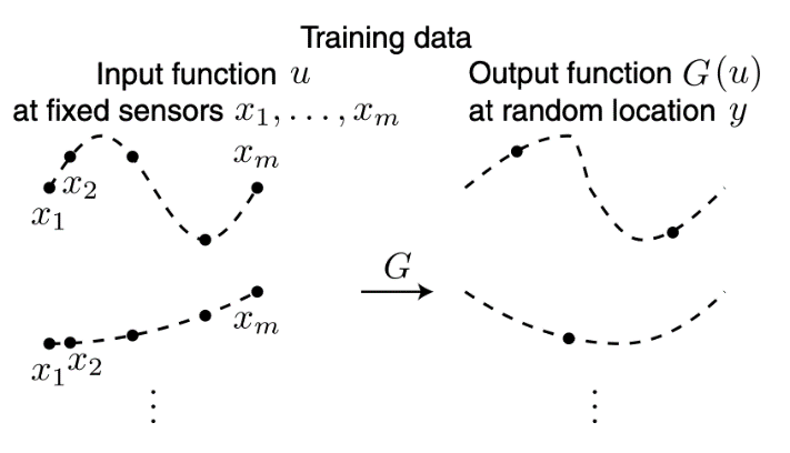
The deep operator network (DeepONet) [6] consists of two deep neural networks, one for encoding the discrete input function space which is a branch net, and another for encoding the domain of the output functions which is a trunk net shown in figure 1. When training the model, the branch net takes the input of function u(x) where the \( xs \) are the sensors fixed on the specific domain, which is shown in figure 2. The trunk net takes input denoted as y of random position on the same domain. Both DNNs output the same amounts of results and then the final predicted result is the inner product of them which is the G(u)(y), where G is the operator taking u as the input function and outputting the target function G(u).

2.2. The proposed framework

The proposed framework is inspired by DeepM&Mnet which is designed to obtain accurate solutions for multi-physics and multi-scale problems in an efficient way. It considerably reduces the computational cost compared with using Autodesk CFD [8]. The main point is to take the locations as the input and then predict the properties of the flow, such as the velocity, the temperature, and the densities of different chemicals [5].

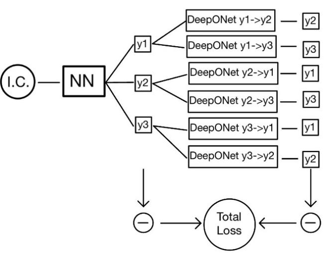
An illustration of our network solving three-dimensional ordinary differential equation system is shown in figure 3. The principle of our model is the assumption that the solutions between dependent variables in a multi-dimensional differential system are fully related. That is, there exist implicit operators between them that we can obtain the other solutions like y2 and y3 here if y1 is known despite unknown initial conditions for a certain ODE system. Although it’s an intuitive assumption without rigorous proof herein, we have attempted to fit a DeepONet model by taking y1 as input and y2 as output to show its feasibility. The NN in the front of the framework is a deep neural network that is trained by loss function from both the measurements (left side) and the operators (right side by DeepONets).

3. Experiment

The solutions for different initial conditions of a certain ordinary differential equations system from a physical problem were obtained to be the training and test data for DeepONets. One solution was used to predict another solution to test the implicit relation between them by the DeepONet. Two solutions were converted to the forms of the inputs and the outputs in DeepONet for training the model with some hyperparameters. This section first shows the experimental settings (Sec. 3.1) used in this paper, and then describes the results and related analysis (Sec. 3.2).

3.1. Experimental Settings

3.1.1. Benchmark Problem. The ordinary differential equation system chosen to test the relation among solutions comes from the ROBER problem [9], a classical stiff chemical kinetic problem that is universally used to test stiff ODE integrators [10]. As in equation (1), The coefficients of the ODE system are simplified for the generation of training data. The y1 is used as input and y2 is used as output to test whether the implicit relation between solutions of this system exists and can be well predicted by DeepONet.

\( \frac{d{y_{1}}}{dt}=-{k_{1}}{y_{1}}+{k_{3}}{y_{2}}{y_{3}} \)

\( \frac{d{y_{2}}}{dt}={k_{1}}{y_{1}}-{k_{2}}y_{2}^{2}-{k_{3}}{y_{2}}{y_{3}}, \)

\( \frac{d{y_{3}}}{dt}={k_{2}}y_{2}^{2}, \)

\( {k_{1}}, {k_{2}}, {k_{3}}=4, 3, 1\ \ \ (1) \)

3.1.2. Implementation Details. Solutions were generated given randomly generated initial conditions with y1(0), y2(0), and y3(0) from 0 to 1. For each solution obtained with a specific initial condition, the y1 and y2 were formed as in picture 2. The input function y1, values of it on fixed sensors ranging from 0 to 1 with the same interspace were the inputs of the branch net. 10 random locations and their corresponding values of y2 were obtained to be the inputs of trunk net and the outputs for each initial condition. There were total of 100000 data points generated and 10000 for training and 90000 for testing. For the neural network DeepONet, we used the following parameters:

• Hidden layers for both branch and trunk neural networks: 40×40.

• Activation function: ReLU.

• Learning rate: 0.001.

• Epochs: 80000.

3.2. Results

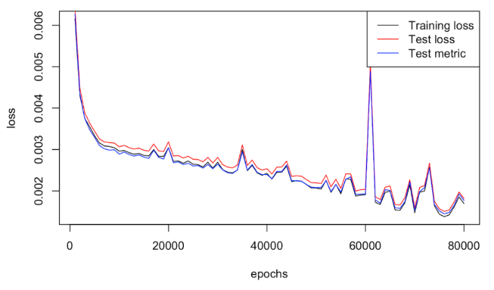
The training loss, test loss, and test metric were recorded for every 1000 epochs. The loss with respect to epochs shown in figure 4 shows that they continued decreasing when there are 80000 epochs. The training loss and test loss of the final model were both 0.00125. It was also conducted with 50000 epochs at first which owned a larger loss as here shown in figure 4.

Some initial conditions were chosen to test and illustrate the result of the model, which are shown in figure 5-7. The red lines were the y2 predicted by y1 which were obtained by numerical method and the black lines were y2 obtained by numerical method.

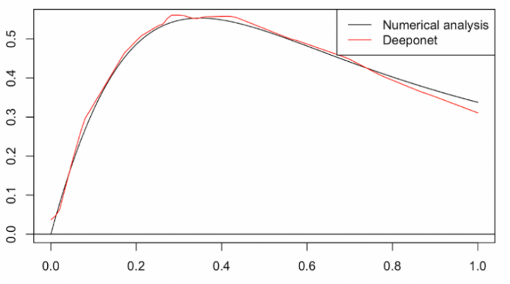
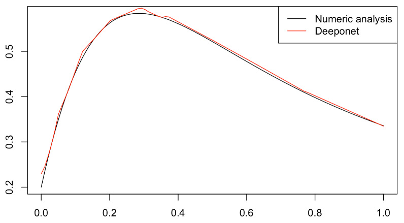
The downtrend of loss for 80000 epochs implies that the model is not overfitting and more epochs are required to reach its best. According to the results in figures 5 and 6 of 50000 epochs and 80000 epochs with initial condition {1,0,0}, the result predicted by the DeepONet agrees more and more with the result from the numerical method as the epochs increase. The results predicted by DeepONet are basically consistent with the numerical results according to figures 6 and 7. There are also some limitations. The predicted results oscillate around the extreme point which is not smooth as the numerical results. There is also incongruity at the beginning points. The overall behavior of the comparison between predicted solutions by DeepONets and numerical methods indicates there is every reason to believe that operator between these solutions exists and is well modeled by DeepONet.

4. Conclusion

In this paper, the feasibility of the proposed DeepM&M-wise net in solving certain DE systems is verified. The relationship among solutions of a certain ODE system is tested to exist and they can be well modeled by DeepONets. Further work is required in terms of obtaining the best DeepONet models and testing the final proposed model. The best model needs to be obtained by increasing the number of epochs for all the DeepONets. Then train and test the proposed DeepM&M-wise net after obtaining all the building blocks.