Analysis of object recognition trends based on deep learning

1. Introduction

Just as vision is the most important perceptual system for humans, so too is target object recognition technology for computers, which is equivalent to the science of computer "seeing". This science of seeing first originated in the 1950s, when it focused on the analysis and recognition of two-dimensional images, such as optical character recognition, the analysis and interpretation of workpiece surfaces, micrographs, and aerial images. In the 1990s, research into the use of projection invariants in recognition, mainly to address projection reconstruction, and numerous successes in areas such as multi-view geometry and camera calibration, saw computer vision techniques evolve and flourish[1-3]. In the field of computer technology before the advent of deep learning, computer vision technology developed based on human-set rules and did not achieve autonomous recognition, and it was the emergence of deep learning technology that pushed target object recognition technology to a brand new stage, and after entering the deep learning stage, computer vision technology was widely applied to many areas, such as in security, autonomous driving, robotics and other In recent years, the alternative technique of Denoising Diffusion Probabilistic (Diffusion Model) has become more and more popular and the quality of the synthesized images is getting higher and higher [4-7].

2. Methods

2.1. Development process

The methods of the technology has gone through the following main stages:

• Traditional detection methods for feature extraction and feature classification using sliding windows and extractors.

• Region-based Convolutional Neural Networks (R-CNN) series algorithms.

• You Only Look Once (YOLO) series algorithms.

• Single Shot MultiBox Detector (SSD) algorithm.

• Diffusion Model [8].

The performance of object recognition algorithms is usuallly judged by the following parameters:

• Recall rate (RR): The proportion of positive cases in the sample that is correctly predicted.

• Average Precision Mean (mAP): Performance metrics for a class of algorithms for predicting target locations and classes.

• Mean log-miss rate (MR^-2): Mean value of the Average Precision (AP) for all species.

• Pre-pass time consumption (ms): Time consumed for the entire process of an image from input to output.

• Frames per second (FPS): The time taken to process an image, used to evaluate the speed of detection.

• Floating point operations (FLDPs): A measure of the hardware standard for floating point numbers running per second.

2.2. Traditional detection algorithms

Object recognition is a very popular area of computer vision research, and due to the limited state of the art in the 1970s, object identification technology did not formally come into its own until the 1990s. It is not difficult for the human eye to recognize colorful objects, but for a computer, faced with a multitude of pixel points, combined with a mixture of object pose, illumination, and complex backgrounds, object recognition becomes more difficult. In the field of traditional detection algorithms, a Histogram of Oriented Gradients (HOG) + Support Vector Machine (SVM) is an example, which is generally used for face recognition [9]. The basic idea can be summarized as that the image is separated into many small connected regions, i.e. cells, and then the gradient amplitude and direction of the cell cells are voted statistically to form a histogram based on the gradient characteristics, and the histogram is normalized over a larger range of the image (aka interval or block), and the normalized block descriptors are called HOG feature descriptor. The feature descriptors of all the blocks in the detection window are combined into an ultimate feature vector, which is then used to perform binary detection of targets and non-targets using an SVM classifier [10]. The algorithm has many limitations, as the feature descriptor acquisition process is complex and has a high dimensionality, resulting in poor real-time performance, it is difficult to deal with occlusion problems, and it is not easy to detect large human pose movements or object orientation changes.

2.3. R-CNN

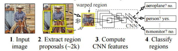
The full name of R-CNN is called region with CNN features, and in fact this full name is an intuitive explanation of the extraction of features by CNN in Region Proposals, followed by classification and regression, the process from providing image information to region classification is shown in figure 1.

The RCNN algorithm is a neural network-based object recognition and detection algorithm, and is highly regarded for its excellent performance and is widely used in various areas of life. The subsequent development of (Faster Region-based Convolutional Neural Networks) Faster R-CNN, Spatial Pyramid Pooling in Deep Convolutional Networks (SPPNet), and Fast Region-based Convolutional Neural Networks (Fast R-CNN) are all based on the R-CNN algorithm and improved along the lines of this model. R-CNN is made based on the AlexNet network and the steps of the R-CNN algorithm are mainly: First determine the possible candidate regions in the detection target,generally find 2000 candidate regions by default (for a single image), where the length and width of the selected 2000 candidate boxes are not fixed and cannot be directly input into the Convolutional Neural Network (CNN). Table 1 is a comparison of the performance of the various methods of selecting candidate boxes. These candidate regions are size-transformed and fed into AlexNet to obtain the feature vectors, and the final output is a 2000*4096 dimensional matrix in the process.

After determining the appropriate method for selecting candidate frames and the size transformation of the image, the next step is to perform the image classification for the candidate regions, which focuses on classifying the image using an SVM classifier, for example, SVM is a binary classifier for A. The binary classification is performed on 2000 feature vectors to determine whether they belong to A. Each classifier will make a judgment on 2000 candidate regions are judged, and so on, to get 2000 candidate region scores, the probability of belonging to A. If SVM is a B classifier, similarly, the probability of having 2000 candidate region scores that belong to B can be obtained, which results in a scoring matrix of [2000,20].

Table 1. Comparison of relevant methods for candidate box selection. (Reference: https://blog.csdn.net/fenglepeng/article/details/117368102.)

Filter the candidate areas to retain only the optimal boxes of the marked objects in the image to exclude redundant interference. As for the filtering process, the computer keeps those with high scores and removes those with low scores, based on the probability of each candidate region's score. For the remaining candidate frames by Intersection over Union (IoU), through multiple iterations, each candidate frame eventually obtains its corresponding Ground truth [11].

In order to obtain more accurate labeling of the candidate frame, a box regression algorithm is performed so that the final candidate frame is closer to the Ground truth. Where assuming that C is the candidate frame and R is the target regression frame, let C and Z do regression training to obtain the parameter P, from which a new operation is performed, i.e. P (Cx, Cy, Ch, Cw) = (Z's, Z's, Z's, Z's),this (Z's, Z's, Z's, Z's) ≈ (Zx, Zy, Zh, Zw), and the new prediction frame is obtained.

R-CNN has a great advancement in detection speed and accuracy compared to traditional object detection algorithms, but there are also obvious shortcomings, training R-CNN is divided into several steps, including region selection, training a convolutional neural network (SoftMax classifier, log loss), training SVM (hinge loss) and training regressor (squared loss). This spends a lot of time and occupies a lot of memory space. While training the convolutional neural network, each region of this convolutional network is to be computed, which generates a lot of redundant computations.

2.4. Fast R-CNN

The way the Fast R-CNN selects the 2000 suggestion frames is still determined by selective search, however, the difference is that instead of feeding these suggestion frames directly into the convolutional network, the raw image is input into the convolutional network to get the feature map, and the suggestion frames then start extracting features from the feature map. The advantage of this is that the original suggestion frames overlap very much and the convolution is heavily double-computed, after the improvement, only one convolution is computed at each position, which greatly reduces the computation. At the same time, Region of interest pooling (Rol pooling) is proposed, integrating bbox regression, classifier, Convolutional Neural Network, and other modules into one, which greatly reduces the computer running time. Where R-CNN uses an SVM classifier, Fast R-CNN uses SoftMax for classification and is computed with a kind of 4x4=16 box number.

2.5. Faster R-CNN

A faster R-CNN algorithm based on region candidates, which unifies the basic steps of target candidate frame selection, feature vector extraction, candidate frame classification, and filtering within a deep network framework, can be deemed to Region Proposal Network (RPN) + Fast R-CNN, which is one of the more advanced object identification models [12]. the purpose of the RPN is to create candidate regions, and then judge whether the target image is background or foreground by the SoftMax classifier, and finally make corrections to get more accurate proposals, and then provide the default 300 candidate Rol pooling and continue to perform the same remaining steps of Faster R-CNN [13].

The Faster R-CNN algorithm, compared to the previous R-CNN algorithm and the faster R-CNN algorithm has significant progress in detection performance compared to the previous R-CNN algorithm and fast R-CNN algorithm, but still has shortcomings, in the recognition of objects with small accuracy and the slow detection of large models. Table 2 reflects the comparison of the three in terms of feature extraction, classification, and testing time.

2.6. YOLO algorithm

The YOLOv1 algorithm, for example, is a typical first-order algorithm that transforms the detection problem into a regression problem, allowing for real-time detection of video, and is widely used. the YOLOv1 algorithm consists of Google Inception Net (GoogleNet) + 4 convolutional + 2 fully connected layers, the core idea is that, after convolutional networks, the image is output into 7x7 = 49 grids, the 49 grids are called grids, and each grid predicts 2 bounding boxes, which one of these two bounding boxes should be chosen? It is decided by the IoU between the box of the object selected by the network and the box of the actual object, leaving the one with the larger IoU as the bounding box, the bounding box is used to predict whether the object exists or not, i.e. the confidence target value is 1, and the position of the real bounding box of the object is also filled in the bounding box, the other one is not The YOLOv1 algorithm can generate a conditional probability of belonging to a certain category, and then multiply each bounding confidence by each conditional probability to obtain the probability of each category of each bounding box, and finally achieve the prediction result [14].

The YOLOv1 has a great advancement in detection speed and precision compared with the previous R-CNN algorithm, but considering the biggest shortcoming of the algorithm itself, due to the increase of the grid point limit and the fact that each grid point can only output one prediction result, the recognition effect is not very good for some small objects in the vicinity. Therefore, based on YOLOv1, the new YOLOv2 algorithm and YOLOv3 algorithm have made corresponding improvements in various aspects such as detection speed and accuracy as well as close object recognition.

Table 2. Comparison of the effects of R-CNN, Fast R-CNN, and Faster R-CNN.

(Table credit: Original)

2.7. SSD algorithm

The SSD algorithm, which emerged later, has good performance with high detection speed and accuracy. The Default Box was introduced in SSD, which is similar to the anchor box mechanism in Faster R-CNN, setting some target preselection boxes, the difference is that the Prior Bounding Box (PriorBox) layer is used on all feature points of the feature map at different scales. Similarly, unlike YOLO, which uses a fully connected layer at the end, SSD makes use of convolution straightly on diverse feature maps to extract detection results, balancing the advantages and disadvantages of YOLO and Faster R-CNN, i.e. Faster R-CNN has higher accuracy mAP and lower miss detection rate recall, but is slower. YOLO, on the other hand, is faster but has lower accuracy and miss detection rates.

2.8. Diffusion model

After the above introduction of algorithms such as R-CNN, YOLO, and SSD, an alternative model algorithm, with a raw mathematical concept, is germinating quietly in different application areas (e.g. protein structure design, text generation), at a time when object recognition techniques are taking the world by storm [15].

Unlike previous object detection algorithms, the diffusion model is learned by a stationary process using probabilistic diffusion theory, and the intermediate hidden variables have a high dimensionality concerning the original data [16,17]. The overall diffusion model is divided into two processes: one is

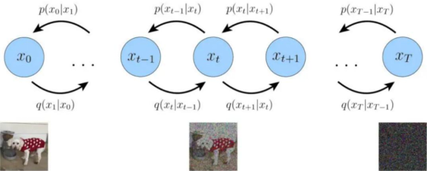
the diffusion process from the target distribution x0 to the noise distribution (also known as the entropy increase process), which continuously adds noise to the original noise and eventually becomes each independent Gaussian distribution. The second is the process of gradually predicting the target distribution from the noise distribution, also known as the inverse diffusion process, where the target distribution is continuously sampled from the noise distribution to extract the target distribution and generate the image, and the process of deriving a large number of mathematical equations is not overly detailed, and the figure 2 is a visual representation of a Variational Diffusion Model, x0 represents true data observations such as natural images, represents pure Gaussian noise, and xt is an intermediate noisy version of x0, each q(xt|xt-1) is modeled as a Gaussian distribution that uses the output of the previous state as its mean.

Diffusion models are easy to handle and flexible, solving the problem that ease of handling and flexibility are two conflicting issues in generative modeling. Easy-to-handle models can perform analytical evaluations and fit data, but they cannot easily describe the structure in a rich dataset. Flexible models can fit arbitrary structures in the data, but the cost of evaluating, training, or sampling from these models can be high. Despite the excellence of the diffusion model, there are some minor drawbacks; it relies on a long Markov diffusion step chain to generate samples and can therefore be costly in terms of time and computation, and although new methods have been proposed to make the process faster, the overall process of sampling is still slower than Generative Adversarial Network (GAN).

3. Results

The following table 3 shows the comparison of R-CNN, YOLO, and SSD algorithms in terms of mAP, FLOPs, FPS, and other related performances. It can be seen that as computer technology continues to evolve, object recognition algorithms have improved greatly in terms of speed and accuracy, as well as detection methods and feature extraction.

In summary, R-CNN has greatly improved the detection speed and accuracy, but still has disadvantages such as multiple training, high spatial and temporal value, and slow prediction phase.

Fast R- CNN improves the testing accuracy and speed of training models, and the input images no longer do selective research but are directly input to the network, which both speeds up the feature extraction and saves storage space, even so, the detection speed is still slow. Faster R-CNN achieves object detection performance with higher accuracy through the two-order network with RPN, especially embodied in small objects with small accuracy and multiple scales, but there are disadvantages such as accuracy loss in Rol Pooling and full connectivity. YOLO was introduced, and the regression algorithm was used to improve the object detection speed, but for small objects, the accuracy of YOLO is not satisfactory. SDD algorithm runs at a higher speed and detection accuracy, but it is difficult to recover from data loss.

4. Recommendations

Although object detection algorithms have improved considerably in the last decade, there is still a long way to go. In the future, hoping that mAP can reach ninety percent and that FLOPs and FPS can also be improved to a higher level. At the same time, how to ensure that the detection speed is faster under the premise of higher detection accuracy and application on some resource-constrained front-end devices; how to find a solution to the problem of occlusion and small-scale detection accuracy; how to perform video object detection, using the redundancy of inter-frame information to accelerate and continuity to improve accuracy; how to use object detection to complete other tasks, solving unsupervised and semi-supervised; how to use object detection to accomplish aother tasks and solve new problems such as unsupervised, semi-supervised, and migration learning; how to further optimize the algorithm level and data processing level of object detection, which are all very critical and hopefully can be solved in the future.

Table 3. Relevant performance comparison of R-CNN, SSD, and YOLO algorithms. (Table credit: Original)

5. Conclusion

This article is an analysis of trends in object detection . The R-CNN , Fast R-CNN , Faster R-CNN , SSD , YOLO and Diffusion model algorithms are introduced , their respective advantages and disadvantages and main features are analysed , as well as the specific problems solved in the process of object recognition . Even though they are already excellent,there are still problems such as data loss,slower speed and lack of accuracy. In order to achieve ultra -high precision and accuracy in object recognition for real -life applications , tools for deep learning need to be further developed.