Neurofibroma detection using joint imaging genomics and ensemble learning

1. Introduction

Neurofibromas can be detected, segmented, and quantified through whole-body magnetic resonance imaging (WBMRI). There are significant morphological differences among individuals, making automatic detection and segmentation a considerable challenge. Widely applied medical image lesion detection primarily includes the detection of pulmonary nodules/lesions [1][2], breast lesions [3][4], brain tumors [5][6], polyps [7][8], and lymph nodes [9][10]. Huang et al. [11] integrated three target detection models, Faster R-CNN, R-FCN, and SSD, achieving the best performance in the COCO dataset’s object detection challenge of that year. Xu et al. [12] proposed an object detection framework based on ensemble deep learning models. Sirazitdinov et al. [13] integrated RetinaNet and Mask R-CNN models to locate and detect pneumonia areas in X-rays. Jain et al. [14] applied ensemble learning to early brain tumor detection. Sreelakshmi et al. [15] introduced an encoder-decoder-based ensemble learning method for medical imaging.

Precision diagnosis and auxiliary medical assistance based on imaging genomics are gradually becoming powerful tools in smart medicine [16]. The automatic extraction of convolutional features from medical images by CNN models to serve as imaging genomics features has also become possible [17]. However, for tumors or lesion areas with significant heterogeneous differences, there is no unified deep learning model that can fully extract features. In such cases, manually designed and constructed (hand-crafted) imaging genomics features have superior and irreplaceable advantages. To the best of our knowledge from domestic and international technical literature, there are no papers specifically addressing neurofibroma detection in WBMRI. This paper proposes a method for neurofibroma detection in WBMRI using joint imaging genomics and ensemble learning, making the following contributions: (1) Proposing an image enhancement method that combines image sharpening, filtering, brightness adjustment, and contrast adjustment to further highlight the texture features of neurofibromas and surrounding tissues in MRI. (2) Since real-time requirements are not essential for medical detection of neurofibromas, integrating various advanced segmentation and object detection algorithms through ensemble learning. This involves using a weighted boxes fusion (WBF) technique based on test-time augmentation (TTA) under a single model and further integrating multiple models using the dual fusion approach of TTA and WBF. For segmentation, minimum bounding boxes based on segmentation masks are utilized for position calibration. (3) Utilizing multidimensional features obtained from imaging genomics for tumor heterogeneity evaluation to effectively remove false positive tumor areas during post-processing.

This method can effectively enhance the accuracy of neurofibroma detection and is also applicable to detecting tumor and lesion areas in other medical images.

2. Research Method

2.1. System Overview

(a)

(b)

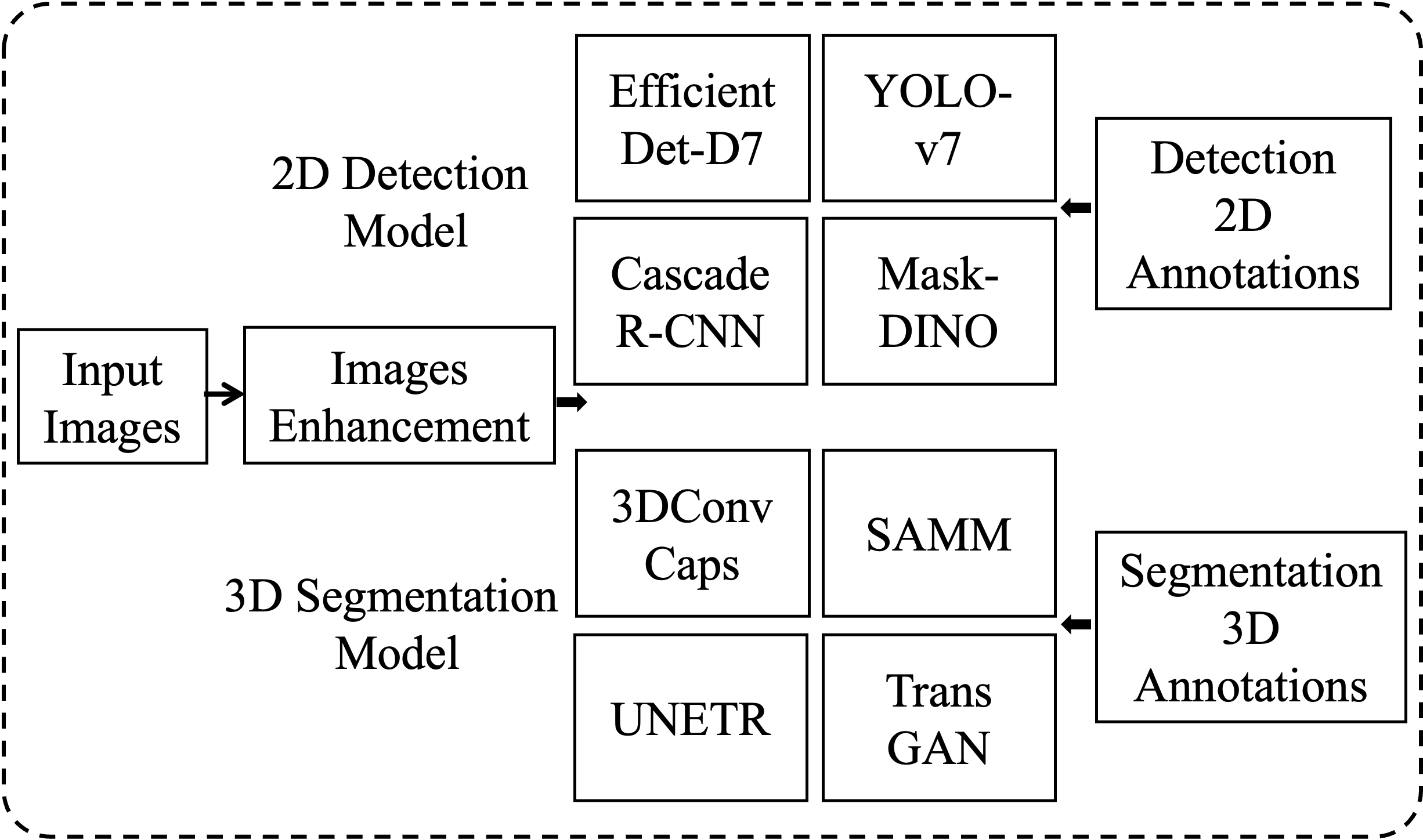
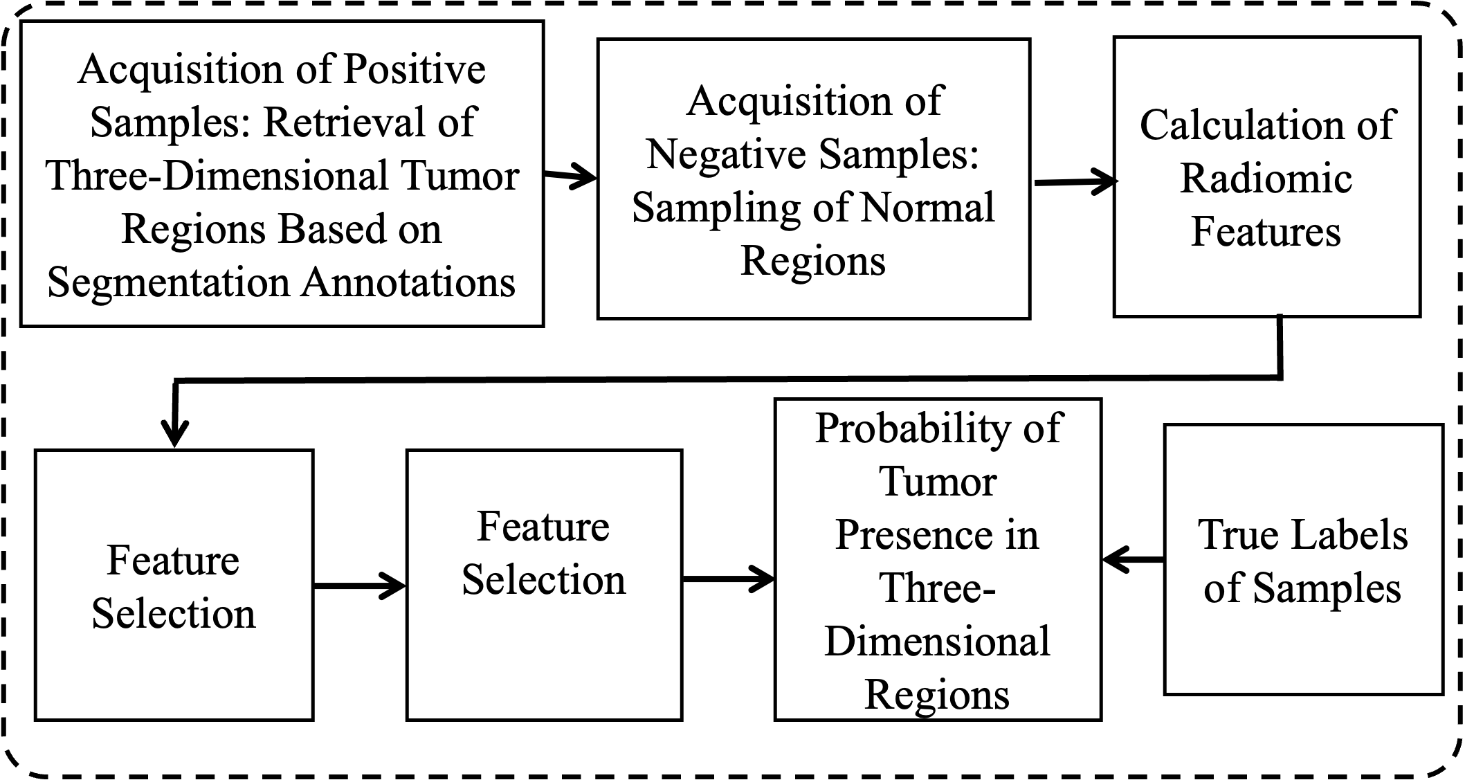
Figure 1. Model Generation Framework. (a) Training independent detection and segmentation models; (b) Training false positive removal classification models.

Figure 2. Ensemble Learning Prediction Framework

The process of neurofibroma detection in WBMRI includes training and prediction. The training process, as shown in Figure 1, involves the independent training of multiple target detection models and segmentation models for ensemble learning, training of false positive removal classification models, and all training processes can be conducted in parallel. For medical image target detection, 2D space is more convenient and efficient, while for segmentation processing, 3D space provides greater accuracy and also supplies 3D data for false positive removal. Prediction, as illustrated in Figure 2, involves integrating and merging the predictions of independent detection and segmentation models. The image enhancement, ensemble learning strategies, and false positive removal algorithms utilizing imaging genomics features are described in Sections 1.2, 1.3, and 1.4, respectively.

2.2. Image Enhancement

Image enhancement can further highlight the structural details and texture features of body tissues and lesion areas in WBMRI, providing more training basis for deep learning. The algorithm process is described as follows:

(1) Input the original MRI grayscale image IM;

(2) Set the total number of times N for operations including image sharpening, median filtering, brightness adjustment, and contrast adjustment, with the current count n set to 1;

(3) Set the minimum and maximum values of parameters lightness and alpha for image sharpening, as well as the increment value for single transformation;

(4) Set the minimum and maximum values of parameter k for median filtering, as well as the increment value for single transformation;

(5) Set the minimum and maximum values of parameter add for brightness adjustment, as well as the increment value for single transformation;

(6) Set the minimum and maximum values of parameter alpha for contrast adjustment, as well as the increment value for single transformation;

(7) Generate all combination values based on the minimum and maximum values of parameters and the increment value, with a total of M combinations, and set the current index i to 1;

(8) Retrieve the parameter combination value for the i-th group;

(9) Perform image sharpening using the lightness and alpha values from the parameter combination;

(10) Perform median filtering on the sharpened result using parameter k;

(11) Adjust brightness of the median filtered result using parameter add;

(12) Adjust contrast of the brightness adjusted image using parameter alpha;

(13) Increment n by 1, if n is less than N, proceed to step (9), otherwise continue;

(14) Output the enhanced image;

(15) Increment i by 1, if i is less than M, proceed to step (8), otherwise continue;

(16) Conduct initial screening by observers on all enhanced images generated by parameter combinations;

(17) Experts make final selections based on the initial screening results;

(18) If the subjective requirements of experts are not met, return to step (2) to reset parameters for enhancement, otherwise continue;

(19) Output the parameter combinations corresponding to images that meet the subjective requirements of experts.

The implementation of image enhancement utilizes the Sharpen method, MedianBlur method, AddToBrightness method, and LinearContrast method in the augmenters interface of the imgaug[18] library for image sharpening, median filtering, brightness adjustment, and contrast adjustment, respectively.

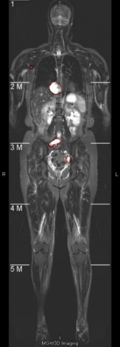
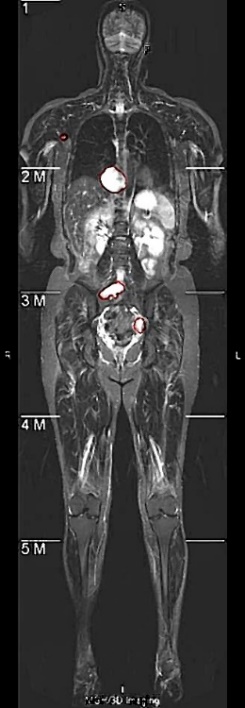
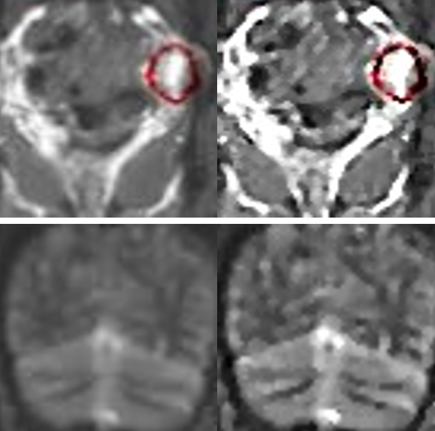
From the overall and detailed enhancement effects in Figure 3, it can be observed that the image enhancement method proposed in this paper effectively highlights the MRI texture details, providing quality assurance support for target detection.

(a) (b)

Figure 3. Comparison of Image Enhancement Effects. (a) Overall comparison; (b) Detailed comparison.

2.3. Ensemble Learning

For detection and segmentation, this paper attempts to effectively combine models based on CNN, GAN, Transformer, and Capsule with significant differences. For 2D object detection models, Cascade R-CNN [19], EfficientDet-D7 [20], YOLO-v7 [21], and Mask-DINO [22] are selected, while for 3D segmentation models, TransGan [23], 3DConvCaps [24], UNETR [25], and SAMM [26] are chosen.

The core idea of ensemble learning is to use a weighted boxes fusion (WBF) based on test-time augmentation (TTA) under a single model, followed by a dual fusion approach of TTA and WBF for multiple models. For segmentation, minimum bounding boxes based on segmentation masks are used for position calibration. The algorithm is described as follows:

(1) The total number of cases in the validation set is N, and each WBMRI case contains M slice images. Set n as the current case, initialized as 1, and m as the current slice image, initialized as 1.

(2) Set the detection model as Di, where 1≤i≤4, with current i initialized as 1.

(3) Apply TTA to the m-th slice of the n-th case, including vertical and horizontal mirroring. Di predicts on both the original image and the transformed image.

(4) All predicted boxes are added to list L and sorted in descending order of prediction probability.

(5) Use the WBF algorithm [27] to merge the predicted boxes, generating \( T_{n}^{m}({D_{i}}) \) , which is the TTA ensemble learning fusion result.

(6) Increment m by 1. If m is greater than M, proceed to step (7); otherwise, return to step (3).

(7) n=n+1. if n > N, go to step (8); otherwise, m is initialized to 1, and return to step (3).

(8) Increment i by 1. Reset n and m to 1. If i is greater than 4, proceed to step (9); otherwise, return to step (3).

(9) Set the segmentation model as Sj, where 1≤j≤4, with current j initialized as 1.

(10) Use Sj for 3D segmentation of the WBMRI of the n-th case.

(11) Compute imaging genomics features for each segmentation area according to the algorithm described in Sections 1.4.2 and 1.4.3 and perform feature selection.

(12) Input the selected imaging genomics features into the false positive removal classification model to determine if the 3D region is a neurofibroma. If not, filter out the segmentation area.

(13) Retrieve the segmentation mask of each slice image in the WBMRI of the n-th case and obtain the minimum bounding box according to the segmentation mask. If the IoU of the false positive bounding box and the \( T_{n}^{m}({D_{i}}) \) predicted box is greater than 0.6, remove it. The resulting prediction is \( T \prime _{n}^{m}({D_{i}}) \) .

(14) The minimum bounding box of true positive regions is the segmentation detection result, expressed as \( P_{n}^{m}({S_{j}}) \) ;

(15) Increment n by 1. If n is greater than N, proceed to step (16); otherwise, return to step (10).

(16) Increment j by 1. Reset n to 1. If j is greater than 4, proceed to step (17); otherwise, return to step (10).

(17) Fuse the TTA fusion ensemble result \( T \prime _{n}^{m}({D_{i}}) \) and the segmentation prediction result \( P_{n}^{m}({S_{j}}) \) using multiple models’ WBF, obtaining the final ensemble learning prediction result \( F_{n}^{m}(D, S) \) .

2.4. False Positive Removal

2.4.1. Acquisition of Training Samples. Positive samples are regions of neurofibromas annotated in the WBMRI three-dimensional space, while negative samples are regions of normal organ tissues outside of neurofibromas. In the experiment, there were a total of 158 cases with 1380 tumors. Using five-fold cross-validation, each training set contained 1104 positive samples, and 1000 negative samples were automatically obtained using the following automated method:

(1) The total number of cases is N, with n as the current case, initialized as 1.

(2) The sampling range is e, with each range increment length set as s, both initialized as 5 pixels.

(3) Obtain the WBMRI of the n-th case.

(4) Randomly select pixels p based on the segmentation annotation mask to obtain the edge of the neurofibroma and the pixel points in the normal area.

(5) Use p as the pixel center and e as the radius to obtain a spherical spatial region as a negative sample.

(6) Set e = e + s. If e is greater than 50 pixels, stop sampling and proceed to step (7); otherwise, return to step (4).

(7) Increment n by 1. If n is greater than N, end; otherwise, return to step (3).

Since the center point p of the sampling can be on the edge of the tumor or in the normal area, these two types of negative samples are selected at a ratio of 50% each.

2.4.2. Calculation of Imaging Genomics Features. Imaging genomics features can form imaging biomarkers in three-dimensional space, providing a comprehensive quantification of the complex internal features of tumors in imaging. Here, seven sets of features are generated, including histogram statistics, gray-level co-occurrence matrix, moments, gradients, runs, edges, and wavelets.

(1) Histogram Statistics: Distribution statistics such as pixel mean, variance, kurtosis, skewness, energy, and entropy in the three-dimensional space of the image.

(2) Gray-level Co-occurrence Matrix: Calculate twenty-two feature values of grayscale spatial correlation by frequency of specified pixel pairs in the space, with bin set to an empirical value of 128.

(3) Moments: Calculate the second central moments invariant J₁, J₂, and J₃.

(4) Gradients: Use Gaussian convolution in three-dimensional space to calculate the mean and standard deviation of gradients in the region.

(5) Runs: Generate texture features of 11 run-length matrices.

(6) Edges: Generate the above five imaging genomics features within 3 pixels of the spatial region boundary.

(7) Wavelets: Combine high-frequency and low-frequency data from three-dimensional wavelet decomposition, calculate the imaging genomics features within the formed 8 wavelet spatial combinations.

2.4.3. Feature Selection. The above seven methods generate 721 different imaging genomics feature values. Relative to the number of training samples, the number of features needs to be further reduced through feature selection methods. The specific process is as follows:

(1) Standardize each feature attribute value.

(2) Calculate the variance of each feature. If the variance is too small, it indicates low feature distinctiveness and should be filtered out.

(3) Calculate the linear and nonlinear correlations between all pairwise features. If the correlation is too high, it indicates high feature redundancy and should be filtered out.

(4) Use seven methods including filter methods, recursive feature elimination, extreme gradient boosting, random forests, gradient boosting decision trees, relevant features, and Lasso regression to rank all remaining features in descending order of importance.

(5) Take the intersection of the top 20 features sorted by each method to generate 13 feature values as the final imaging genomics features.

3. Experiment and Discussion

3.1. Experimental Environment and Data

The experimental hardware environment mainly consists of GPU cards that support deep learning, with the model being NVIDIA Tesla V100, quantity 1. As for the software environment, Ubuntu 16.04 operating system, VSCode development environment, Python as the development language, and TensorFlow, Keras, and PyTorch development platforms are used for single-model deep learning training. The WBMRI image data of neurofibromatosis patients in the experiment comes from a collaboration between Harvard Medical School and tertiary hospitals in China. The dataset includes 158 cases with a total of 1380 tumors, and five-fold cross-validation is performed. The segmentation annotations are completed by domain experts, and the target detection annotations are automatically generated using the minimum rectangular box of the segmentation area.

Each WBMRI sequence includes about 20 DICOM format scan images. For target detection training, the image sequence is first converted to 8-bit grayscale images with the original resolution of 322×1086. Since the width and height of the original images vary, it has been empirically proven in academia and industry that deep learning performs better on square two-dimensional images. Therefore, the images need to be adjusted to squares. The image background is black, and the smaller side of the image is directly padded with the background color value to expand the boundary. After the boundary is expanded, the scanned object does not deform and remains centered in the image. At this point, the resolution is 1086×1086. Then, each scanned image is resized to 512×512, and in three-dimensional space, all are resampled to 512×512×32. After resampling, the single-layer two-dimensional images are enhanced according to the algorithm described in Section 2.2 of this paper, and then the images are normalized. The pixel values of all images are divided by 255 to convert them to a numerical range of 0-1. For 2D target detection, the input image size is 512×512, and random image augmentation is performed during training. The random combinations of augmentation methods include horizontal flipping, vertical flipping, random rotation within 90 degrees, and random scaling and translation within a range of 10%. For 3D segmentation, the input patch size is 32×32×32, and no data augmentation is performed during training.

3.2. Qualitative Analysis and Discussion

Neurofibromas may be distributed to any part of the body, mainly including the legs, arms, head and neck, chest, abdomen, and pelvis. The volume can also vary from a few cc/ml to several hundred. In the following display, 7 representative images will be selected, covering different parts of the body and volumes ranging from 5cc/ml to 500cc/ml. As shown in Figure 4, it is a comparison between the integrated learning method proposed in this paper and the detection results of 8 single-models. Here, GT, ED, YL, CR, CC, DINO, and GAN respectively represent Ground-Truth, EfficientDet-D7, YOLOv7, Cascade R-CNN, 3DConvCaps, Mask-DINO, and TransGAN. All detection results are predicted after being processed by the image enhancement algorithm proposed in this paper. From the display results, it can be seen that the detection results of the integrated learning method in this paper are basically consistent with the Ground-Truth, with only a small amount of difference near the boundary.

3.3. Quantitative Analysis and Discussion

The performance comparison results of neurofibroma detection are shown in Table 1. For five-fold cross-validation, the averages are shown in the table. Compared with all single models, the integrated method proposed in this paper achieves the best results in all performance indicators. Compared with the best-performing 3DConvCaps in the single models, AP(@0.5 IoU), AP(@0.75 IoU), sensitivity, and CPM are higher by 10.1%, 9.1%, 7.8%, and 8.5% respectively. The average number of false positives is reduced by 17.68, approximately 6 times fewer. By combining the dual WBF integrated learning with TTA, the AP value, sensitivity, and CPM can be effectively improved to a certain extent, and a small number of false positives can be removed through a voting mechanism. The significant reduction in false positives is mainly due to the removal of false positives through imaging genomics features in the post-processing.

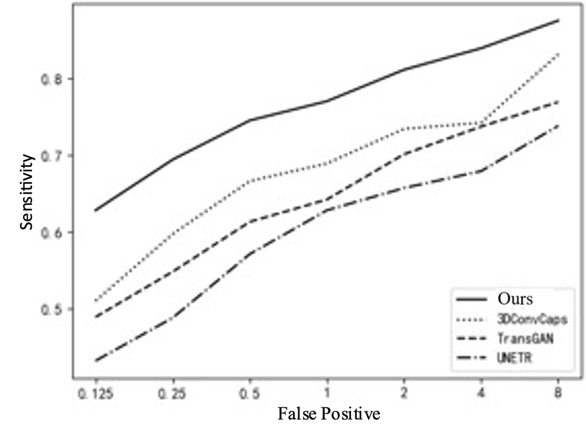
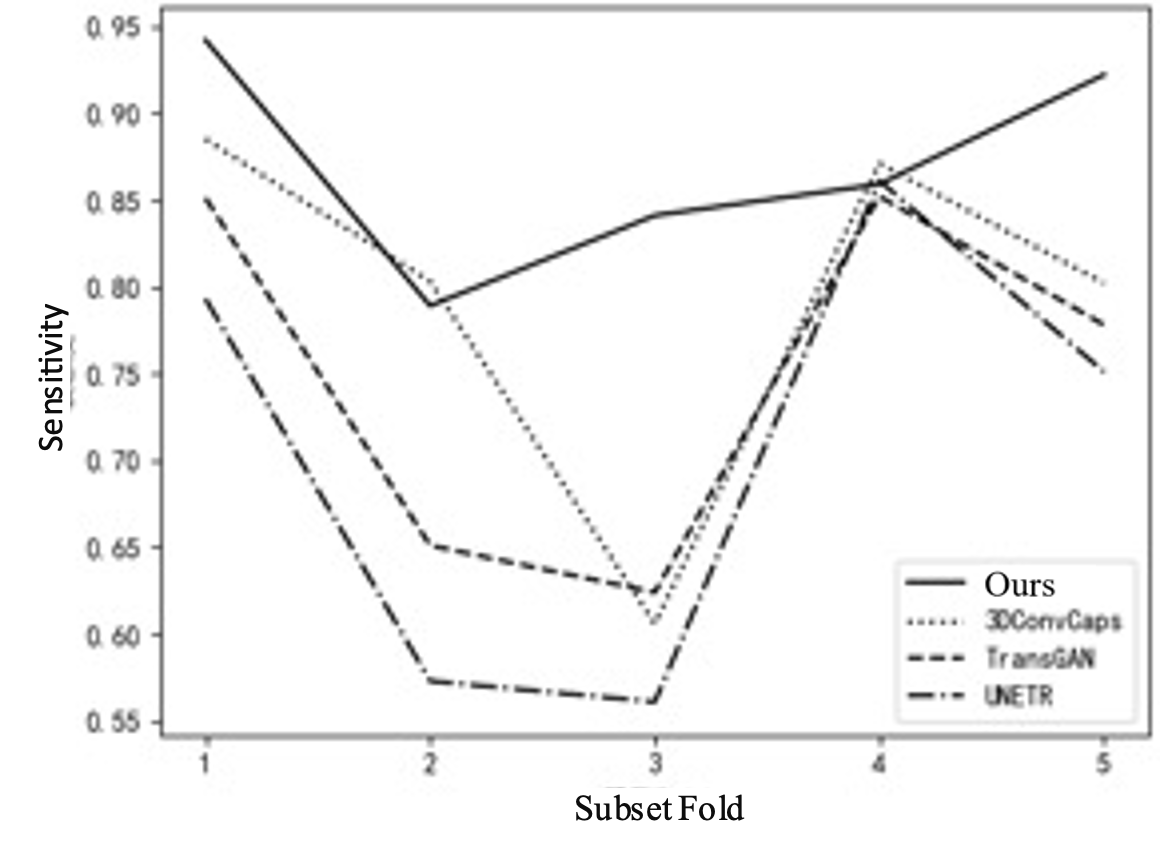
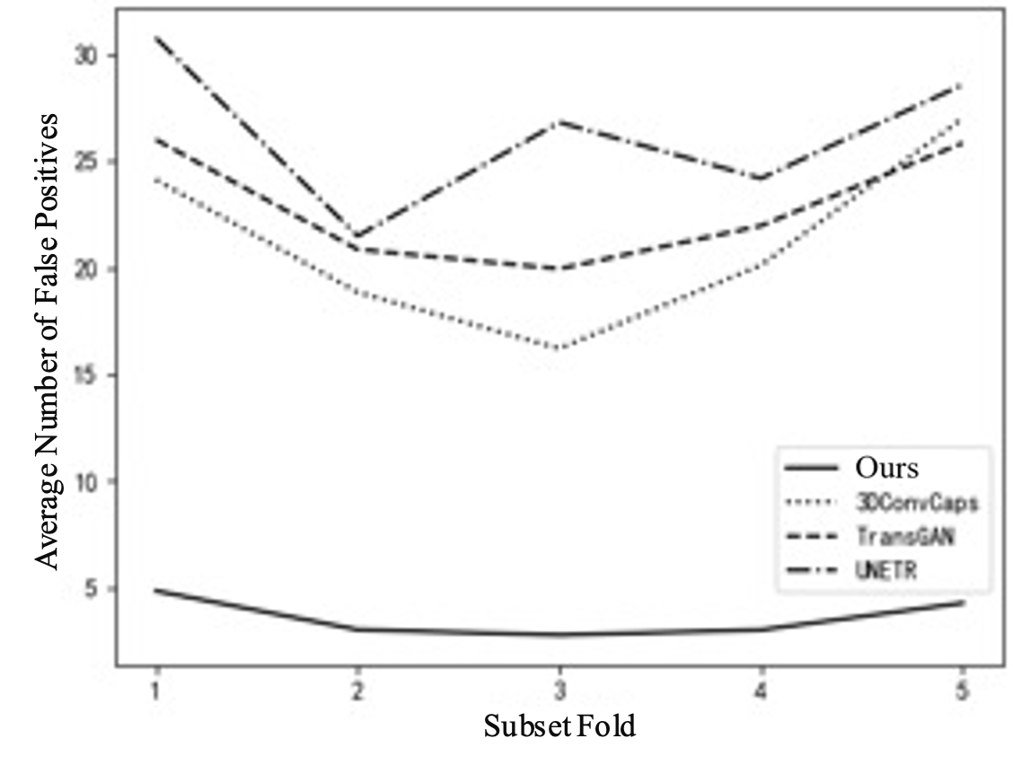
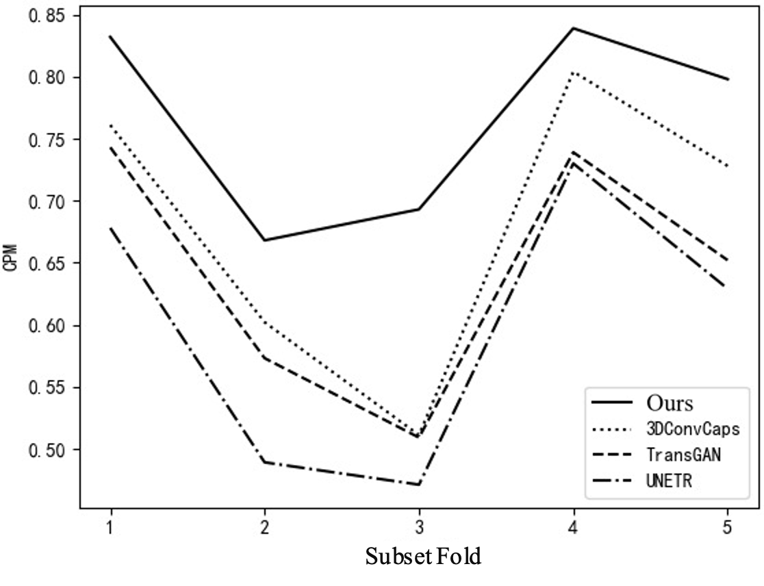
To further explain the results of cross-validation, comparisons between this method and the top three best-performing single models in each fold are conducted, as shown in Table 3 and Figure 5. Comparing with the top three single models can clearly illustrate the issue. If all comparisons are made, the curves in the figure will be too overlapping and unclear. Figure 5(a) shows the FROC curve, with data from Table 1, indicating that the performance of this method is far superior to that of other single models overall. In Figure 5(b), it can be seen that the highest sensitivity of this method reaches 0.942, while 3DConvCaps, TransGAN, and UNETR are only 0.885, 0.852, and 0.793 respectively, which is 0.149 higher than the worst result. In Figure 5(c), the minimum average number of false positives for this method is 2.77, while 3DConvCaps, TransGAN, and UNETR are 16.21, 19.95, and 21.49 respectively, which is 18.72 less than the worst result. In Figure 5(d), comparing CPM, the highest value for this method is 0.839, while 3DConvCaps, TransGAN, and UNETR are 0.804, 0.739, and 0.730 respectively, which is 0.109 higher than the worst result. From the results of cross-validation, the performance indicators on each fold are higher than those of other models, further demonstrating the stability of the model and the significant advantages brought by the integrated method and imaging genomics.

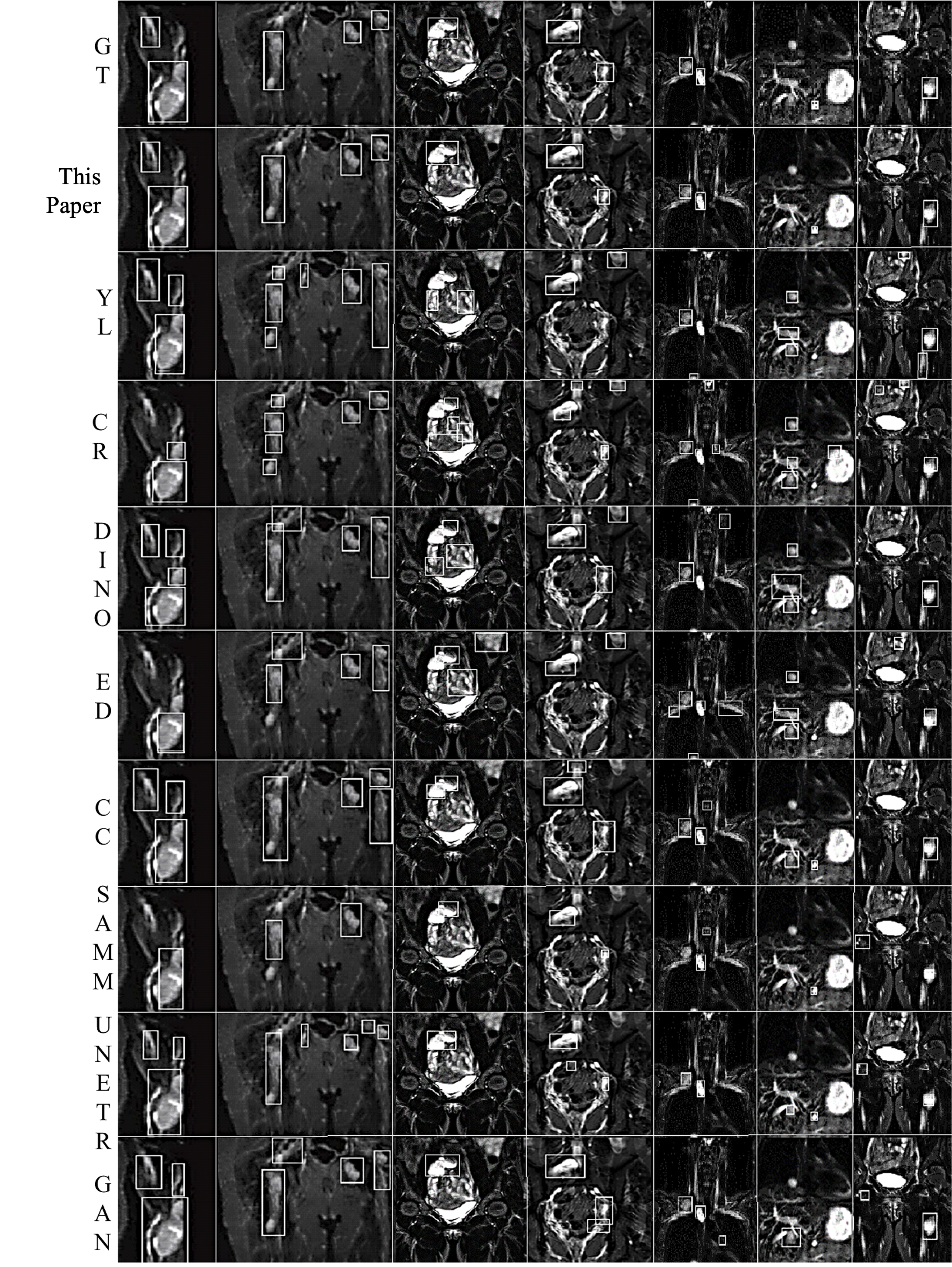
(1) Arm (2) Pelvis (3) Abdomen (4) Abdomen (5) Neck (6) Chest (7) Leg

Figure 4. Comparison of Detection Results by Different Methods

Table 1. Comprehensive Performance Comparison Metrics

Table 2. Cross-Validation Comparison

Table 3. Comparison of Tumor Detection with Different Volumes

(a) (b)

(c) (d)

Figure 5. Line Chart Comparison. (a) FROC Curve; (b) Sensitivity; (c) Average False Positives; (d) CPM

Furthermore, a comparison of tumor detection results based on different volumes is conducted. Due to the adoption of five-fold cross-validation, the analysis is based on the average values of the validation set. There are a total of 276 tumors, with quantities distributed as follows: below 10cc/ml, 10-50cc/ml, 50-100cc/ml, and above 100cc/ml, with 99, 121, 39, and 17, respectively. The comparison results are shown in Table 3. It can be observed that regardless of the volume distribution interval, the performance of the proposed method is the best. The detection proportion in each of the four intervals is higher than the worst result of the single model by 0.15, 0.17, 0.10, and 0.30, respectively, with an overall detection proportion higher by 0.16. Tumors sized between 10-50cc/ml are easier to distinguish morphologically and texturally, leading to the highest detection rate. The average detection proportions for tumors between 50-100cc/ml and below 10cc/ml are close because smaller volumes lead to decreased recognizability, while larger volumes may cause one tumor region to be recognized as multiple, thus lowering the detection proportion, which also explains why the detection proportion of tumors larger than 100cc/ml is lower.

4. Conclusion

Whole-body MRI (WBMRI) three-dimensional imaging is the core imaging method for detecting patients with neurofibromatosis. The complexity in the distribution, morphology, and volume of such tumors throughout the body increases the difficulty of automatic detection. A detection method combining radiomics with ensemble learning is proposed. Firstly, medical images are enhanced to highlight textural features. Then, a dual fusion ensemble learning method, based on single-model test-time augmentation (TTA) fusion, is applied, followed by multi-model weighted box fusion (WBF). Finally, false positive tumor regions are further removed using radiomics features. Experimental results show that the proposed method outperforms the best single-model results in multiple evaluation metrics including AP, sensitivity, average false positives, CPM, and FROC. It can effectively improve the accuracy of neurofibromatosis detection and is also applicable to the detection of tumors and lesion areas in other medical images. Currently, precise segmentation of neurofibromatosis remains a major challenge. In the next research phase, ensemble learning will be combined to conduct automatic segmentation of neurofibromatosis.

Funding

This research is supported by the following funds: the Natural Science Foundation of Ningbo (2023J182), the Ningbo Medical Science and Technology Plan Project (No. 2021Y71), the Ningbo Public Welfare Fund Project (No. 2022S048), the Science and Technology Plan Project of Ninghai County (No. 2106), the Natural Science Foundation of Zhejiang Province (Grant No. LQ21H060002), the Joint Construction Project of Henan Provincial Health Commission (LHGJ20230442), and the Scientific Research Project of Kaifeng Science and Technology Bureau (2303052).