Research on Predicting Customers' Next Purchase Based on Shopping Basket Data

1. Introduction

Thanks to the prosperity of internet technology, online shopping has been popular for people to complete the purchase process online. How to predict customers' next purchase based on shopping basket data is an important problem, which is widely used in online advertising and item recommendation applications [1] [2]. Motivated by this, the goal of this paper is to utilize the market data to guide the market decision, which is proved to have the large potential in numerous studies [3] [4]. Specifically, this paper attempts to find out what products will be purchased by customers in the future. For example, if Lily always purchases food on Sunday and work supplies (for her company) at the beginning of each month, the purchase pattern can be found in her historical purchase data. The more accurate the predictions, the higher the profit. Hence, it is necessary to dig out as much useful information as possible to support the predictions.

In this paper, three types of methods are employed to make the prediction, including the frequency-based method, the rule-based method, and the similarity-based method. These three methods consider the prediction following different ideas. For example, frequently bought items are more likely to be purchased the next time. The frequency-based method takes this idea. Moreover, the evaluations of these methods are conducted on the Instacart groceries dataset and effective conclusions are derived.

In the following, this paper first introduces the research method, and then analyzes the data results obtained by the method.

2. Research Method

This section presents several methods used for shopping basket data analysis and describe the data sources.

2.1. Methods Overview

2.1.1. Data Modeling

The first thing for the next purchase prediction is to model the shopping basket history data of each consumer. For each consumer, his shopping basket history is a series of chronologically ordered sets, where each temporal set is the consumer's purchases at the corresponding time. Formally, the shopping basket history data can be modeled by the following process.

All items that appear in the data are modeled as a set I, i.e., with n items. The shopping history of each consumer is denoted as Bc, which is an order of item collections, . In particular, each item collection contains the items that the customer bought at a corresponding time. Thus, each customer has mc purchase records and the mc of each customer can be different. Then, the shopping basket history data of all k consumers can be represented as .

Formally, the personalized purchase prediction problem is defined as follows [5] [6]. Given a set of items , the purchase history of k customers , where each customer’s purchase history Bc is an order of sequence and , the personalized purchase prediction problem is to predict the purchase of the customer c at the next time, i.e., .

In modern online shopping platforms, there are always numerous items on sale and each customer can only buy at most a dozen items at a time. Therefore, most of the items are not helpful for prediction, and how to identify the truly valid items is the key problem for shopping basket prediction.

2.1.2. Frequency-based Method

Each consumer's personal purchase history faithfully records his preferences. Products that were frequently purchased in the past are likely to continue to be purchased. Inspired by this idea, this paper plans to make predictions based on the frequency of items being purchased. In other words, the more frequently an item has been purchased in the past, the more likely it will be purchased next time.

2.1.3. Rule-based Method

The correlation between products can also help us predict the next possible purchase. Although there is only the id information of products (but no other details) in our data set, this information is also hidden in the data because people consider the relationship between products when making purchasing decisions. A famous example is the story of beer and baby diapers. Although the truth of this story is open to question. It suggests association rules between data. In the next purchase prediction problem, if there are the rules of which goods are more likely to be purchased after the purchase of item A, it will be beneficial to our forecast.

2.1.4. Similarity-based Method

People with similar purchasing experiences will buy similar items in real life. For example, if two mothers have both purchased some baby products in the past, one can recommend each other's shopping items for the other one to make predictions. As a result, it is reasonable to look for similar consumers and goods for purchase predictions. Such an idea is widely used in different fields, such as classification and recommendation [7].

2.2. Details of Methods

2.2.1. Frequency-based Method

The overall process for prediction for each customer is as follows:

(1) Calculate the average number of items purchased by consumers per order (denoted as n_c), i.e., , where m_c is the number of orders in the personal purchase history.

(2) Find the top-n_c frequent items as the prediction results.

In particular, the frequency of each item is the number of times it has been purchased. This idea is widely used in different studies.

For consumers without purchase records, the prediction based on personalized purchase history is invalid. At this point, only the purchase information of all other consumers can be used to make predictions. In other words, one can directly extend the method based on top-n_c to the global purchase history data. Specifically, n_c is the average number of products per order of all consumers, and the calculation of top-n_c items is based on the purchase records of all consumers.

2.2.2. Rule-based Method

As the goal of this paper is to predict the next purchase, the traditional rule-based method is extended for obtaining the rule of which items will be purchased after another item.

The traditional association rule analysis algorithm is based on frequent itemsets, aiming at finding such rules: if item A is purchased, which items are more likely to be purchased? But what the goal is to predict the next purchase. In other words, this rule is required: Which items are more likely to be purchased by a consumer if he previously purchased item A? Therefore, it is necessary to process the purchase history sequence so that it is possible to directly know which items will be purchased after a certain item.

Formally, given any two identical consecutive baskets and , all item pairs can be derived according to Cartesian product, that is, . With the new dataset, all frequent item sets based on the Apriori algorithm can be firstly derived [8]. Then the related rules can be obtained according to association rule algorithm [8]. Finally, the predictions are derived according to the rules and the last item purchased by consumers.

2.2.3. Similarity-based Method

In addition, the predictions based on similar users or similar items are also effective [5] [9]. For a consumer to be predicted, one can either look for consumers similar to her to make predictions, or it is also effective to make predictions based on items similar to the items she often buys.

The prediction method based on similar users is as follows:

1)Calculate the similarity between any two users according to their purchase sequence history.

2)Find the X users who are most similar to the current user.

3)Use the n_c items most frequently purchased by user X as the prediction results.

Since the data set consists of different series, the similarity measure on time series data is employed, e.g., Euclidean distance [10] and dynamic time warping [11]. As Euclidean distance does not support variable-length data, the dynamic time warping is used to measure the similarity of two consumers’ purchase sequences.

The whole process of the prediction method based on similarity of items is as follows:

1)Calculate the similarity between any two items according to their purchase sequence history.

2)Find the n_c items that are most similar to the current purchased items.

For the similarity between items, the frequency of their common purchases is used to measure them, i.e., the number of times items i_x and i_y appear in one order divided by the total number of orders where the two items are purchased (separately or together).

2.3. Data Source

The public Instacart groceries dataset is used in the experiments, which includes 3,214,874 orders with 49,688 different products. Following previous studies, we remove the uncommon items in the dataset and reserve the 500 most frequently used items [5] [6]. After preprocessing, there are 202,821 customers and 500 items. Then the analysis on the filtered dataset is reported.

3. Results and Analysis

In this section, the experiment results and findings are reported. All algorithms are implemented by Python.

First, the sale volume distribution of products bought by a customer is reported. 10 customers are randomly sampled and the purchased times of each item for each customer is counted. Figure 1 depicts the corresponding results of four customers.

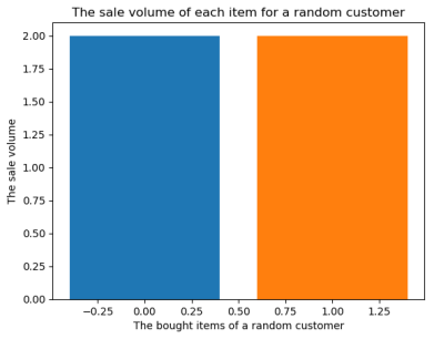
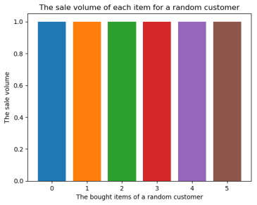
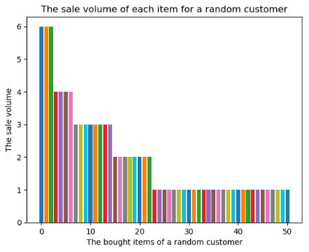
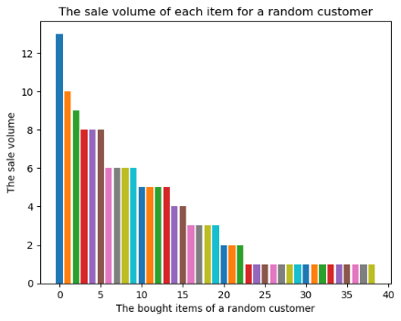
Figure 1: The sale volume distribution of four randomly sampled customers.

In Figure 1, there are some cases (i.e., the first and second figures) where the sale volumes of all items are the same and small. This is because, these two customers only have one or two orders, which contains very less information for prediction. In the extreme case, i.e., there is only one order for a customer (in the second figure). It is impossible for us to utilize such data, since when only one order is used as the purchase to be predicted, there is no order history of this customer for personalization. It tells that, there is a need to think about the general method for forecasting customers with less order history.

In contrast, for the customers with more order history data, the sale volume distributions are shown in the third and fourth figures of Figure 1. These figures confirm our problem analysis. First, there are many items that are never bought by customers. Second, almost half of the items are bought only once. It can be argued that one should pay more attention to the frequently bought items for prediction since they have higher probabilities being bought next time than the ones that are rarely bought or even bought by no one.

Second, the number of products bought in different orders are studied to obtain some intuition for predicting the number of items in the next purchase. Table 1 depicts the results of five randomly sampled customers.

Table 1: The items in an order of five randomly sampled customers.

One can find that, for one customer, his average number of items in all orders is consistent with most of his orders. For customer 66852, the average number of 7.29 is far from the number of items in the last order (12). This is because the number of items he bought at each time are very different. Therefore, it is reasonable to consider the item number per an order as an estimation of the number of items in the next purchase.

Figure 2 shows the item sales distribution of the top-20 items. As can be seen, items such as bananas, bags of organic bananas, and strawberries are items that consumers often purchase at grocery stores. The banana item was purchased over 400,000 times, while the grape tomato was purchased approximately 100,000 times. Figure 3 shows the item sales distribution of the least-20 items. These items were purchased approximately 10,000 times compared to the first 20 items that were purchased frequently. Thus, it can be seen that there is a clear long and short tail effect in the distribution of item sales. Therefore, using the frequently purchased items for prediction is reasonable.

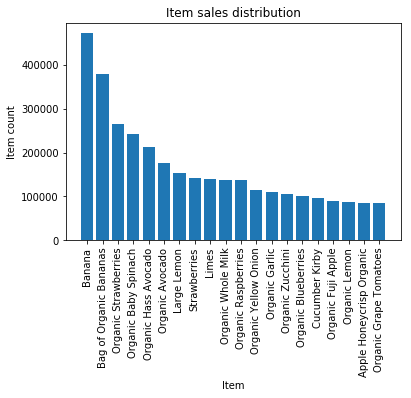
Figure 2: The item sales distribution of the top-20 items.

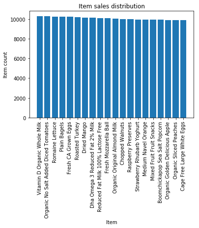
Figure 3: The item sales distribution of the top-20 and last-20 items.

Now let's look at a few of the most frequently purchased items and the last purchased items by consumers. Table 2 shows the most frequently bought items of 5 sampled customers. The items in bold are the ones that appear to be the top-10 most frequently bought items for that customer.

Table 2: The most frequently bought items of 5 sampled customers.

As you can see from the table, the last item that the user purchased, i.e., the item that needed to be purchased, was also frequently purchased before. For example, the last item purchased by consumer 94584 was exactly the same as the previous one, and 5 of the 8 items last purchased by consumer 66852 appeared in the top 10 most frequently purchased items by that consumer. This justifies the use of frequency-based prediction methods.

At the same time, there are cases where the last goods purchased by the consumer differ significantly from the collection of goods purchased frequently before. This may be because consumers are interested in new items and the frequency does not capture this effectively.

Moreover, the overall performance of all algorithms is evaluated for meaningful conclusions. The following metrics are employed to quantify the effectiveness of the above methods.

F1 score: The F1-score is defined as the harmonic mean of precision and recall and is a common metric for market basket comparison.

Jaccard coefficient: The Jaccard coefficient is the ratio of cooccurrences to non-co-occurrences between items of the predicted market basket b and items of the true next market basket b^*. Formally, the Jaccard coefficient is defined by 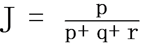where p is number of items in both b^* and b; q is the number of items in b^* and not in b; and r the number of items not in b^* but in b.

Table 3: Experimental results on Instacart groceries dataset.

(F1 data sources: https://en.wikipedia.org/wiki/F-score Jaccard coefficient data sources: https://en.wikipedia.org/wiki/Jaccard_index).

As shown in Table 1, the personal top items have the highest accuracy. It confirms the idea of employing personal data for prediction. Compared with the personal top items, the global top items obtain a less accurate score. This is because, the global information is not suitable for the personalized next purchase prediction, where each customer may have different preferences. The associated rule-based method performs worse. This may be because the rules obtained are not enough to predict the items purchased the next time. The reasons may be two-fold. First, this method is designated for finding the items that are always purchased together, which mean they are not “order-sensitive”. Second, only the “neighboring” (i.e., 1-hop) basket is considered, where the associated shopping baskets in the real world may not be adjacent.

The predicted items based on similar users can achieve comparable performance to the personal top items. The reason is that the items of similar users are also similar to their personal top items, where the similarity between users is computed based on these items. The last purchased similar items have less accuracy than the items from similar users. This is because the item similarity measurement is not as good as the dynamic time warping measurement on users.

4. Conclusions

In this paper, we study the problem of predicting the items in the next purchase, given the historical data of the customers’ baskets. We analyze the problem and the real-world dataset and propose three types of methods to deal with it, including using the frequent items as prediction, associated rule-based prediction, and similar users/items-based prediction. It is found that the frequency-based prediction can achieve high accuracy. The rule-based method is not capable of finding the accurate items in the next purchase since it was not originally designated for the next purchase prediction problem. The predicted items from similar users can also obtain comparable performance. The prediction accuracy of the proposed methods still has much room for improvement. In the future, it is promising to consider the correlations between items and users and employ neural networks to learn the representations of items and users for better prediction.