Research of the Influence Factors of Housing Price-Take Singapore as an Example

1. Introduction

Global housing prices have risen steadily for years, and this pushes up the cost of living for many people around the world [1]. In Singapore, the housing prices have experienced significant fluctuations. From 2006 to 2012, both the Housing Development Board (HDB) flats and the private residential property prices rose steeply before stabilizing [2]. From 1980 to 2015, the average annual housing prices in Singapore for the private sector has a growth rate of 7.02% while for the secondary public housing sector is 6.81% [3]. Since 2020, prices started to climb sharply once again, due in part to the COVID-19 pandemic [4]. As a result, the rising prices directly affect the expenses of individuals and families, making it more challenging to meet their housing needs. However, the public does not realize the influencing factors of housing prices. Hence, this article aims to use the Singapore housing price research to help people assess the expected purchase of a house based on the different underlying factors that may contribute to the house price.

Some researchers are studying the factors influencing housing prices. To track the price reaction of existing homes to the quantity of new units introduced by Singaporean home builders, Joseph and Thao used Vector Autoregression (VAR) models. They discovered that marginal supply Granger-cause current home prices favorably, defying the negative reaction predicted by the "competition" concept [5]. However, the data that they used was from 1996 to 2009. The result may be out of date, which will lower the accuracy of the results. Bian et al. applied econometric analyses and machine learning approaches, using a hedonic model, least absolute shrinkage and selection operator (LASSO), random forest, and artificial neural networks to get deeper insights into the importance of determinants of property prices [6]. They find that property prices are mostly affected by key macroeconomic factors, such as the time of sale, the size, and the floor level of the property. The machine learning approaches that they used can give them more accurate predictions.

Similarly, Cheng and Liu analyzed the effects of macroeconomic factors, supply factors, and alternative housing prices on housing prices in Singapore [7]. They used the two-stage least squares method to estimate the regression equations for the public resale market, condominium, townhouse, semi-detached, and detached housing markets. Tu modified the dynamic stock-flow model and applied it to the Singapore private housing market [8]. Yong got the result that the movements in the real (Gross Domestic Product) GDP per capita and the total housing stock were found to significantly impact real housing prices in the long run. Zhang et al. got the survey results of a positive correlation between property cost and housing price [9]. However, it just focused on the private housing market, and the results may not be suitable to be used in the HDB market. Gang et al. used the decision tree approach, examining the relationship between house prices and housing characteristics [10]. They find that housing characteristics are a factor influencing the housing price.

Thus, this essay will apply the multiple linear regression model to learn the effect of these six factors on the resale price of houses in Singapore. This paper focuses on six variables (Flat Type, Storey Range, Floor Area, Remaining Lease, Lease Commence Date, and Flat Model) and further finds a suitable model to find the relationship between these factors and housing prices.

2. Methodology

2.1. Data Source

The data is extracted from the website Kaggle for dissertation. The data set of the housing price from 2017 to 2022 was published by Singapore's Housing Development Board (HDB). The data includes 10 types of metrics such as month registered for resale, town, flat types and flat area in Singapore. There are 134168 groups of data in the dataset, this survey chooses 3000 of them as samples.

2.2. Variable Description

The housing price will be predicted based on the following 6 variables, which are showed by the Table 1. The ranges of these variables are also showed in the table. In this research, 6 variables are chosen, they are flat type, storey range, floor area, remaining lease, lease commence date and flat model. Apart from that, the independent variable is the release price.

Table 1: The variables used in the model

2.3. Model Instruction

Multiple linear regression is used to find the influencing factors. There is a dependent variable, resale price of the house, and five independent variables, room flat type, storey range, floor area, remaining lease, lease commence date and flat model. This paper aims to analysis how the six factors (X) influence the house resale price(Y) by using multiple linear regression. The equation can be generated:

\( y={β_{0}}+{β_{1}}{x_{1}}+{β_{2}}{x_{2}}+{β_{3}}{x_{3}}+{β_{4}}{x_{4}}+{β_{5}}{x_{5}} \) (1)

3. Results and Discussion

3.1. Data Analysis

Table 2 shows the analysis of the original data, giving minimum and maximum values, mean, median and standard deviation of each variable.

Table 2: Descriptive data

3.2. Correlation Analysis

As can be seen from the Figure 1 and Table 3, correlation analysis was used to study the correlation between six items resale price and storey range, flat type, floor area, remaining lease, lease commence date and flat model. Pearson correlation coefficient is used to indicate the strength of the correlation.

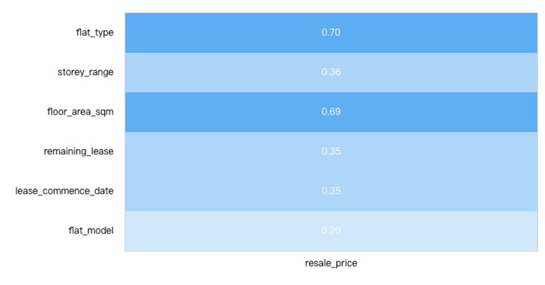
Figure 1: Pearson correlation visualization

All of the six variables have positive correlation with the resale price (dependent variable), and they all have the level of 0.01 significance. From Figure 1, both \( {X_{1}} \) and \( {X_{3}} \) have higher correlation values relatively, with the value of 0.70 and 0.69 respectively.

By testing the multi-collinearity of six variables, it is clear that in Table 3 most of them are not closely related. Nevertheless, there are still some variables that are correlated to others. Take \( {X_{4}} \) and \( {X_{5}} \) as an example, the multi-collinearity is 0.999, indicating that \( {X_{4}} \) and \( {X_{5}} \) are similar to each other, and they influence the result of the model. Hence, it is necessary to delete one of them when modeling. (For convenient, only show \( {X_{4}} \) and \( {X_{5}} \) ).

Table 3: Multi-collinearity 

3.3. Liner Regression Model

Table 4 shows the relationship of six factors and the house resale price. Variables with VIF higher than 5 mean that they are highly correlated to each other. Lease commence date and remaining lease have VIF value higher than 5, suggesting they are correlated. One of them should be eliminated to improve the model. By focusing on the p value, lesser the value of p, more the significant of variable is. Those with p value higher than 0.05 mean that they are insignificant and will not influence the dependent variable. Table 4 suggests that flat model, lease commence date and remaining lease are not significant.

To improve the model, the insignificant and correlated variables are eliminated. In table 5, all variables’ p values are equal to 0, which shows that they are significant and will influence the resale price of houses in Singapore. The VIF values of them shows that are all below 5, which means that they are not correlate to each other. By looking at their B values, storey, flat area and remaining lease have positive influence on the resale price while flat type has a negative influence. With the increase storey and flat area, the resale price will increase. The remaining length of lease means how long they can own their houses. The longer time they can own, the higher the resale price. The flat type is also known as room allocation. The number of rooms increases will cause price to decrease. Compared to the previous model, the regression coefficients have changed slightly. There is no covariance issue in the improved model. The relationship can be explained in the following equation.

\( Y=-6236.981{x_{1}}+9622.849+44877.685{x_{3}}+2512.839{x_{4}}-162082.198 \) (2)

The \( {R^{2}} \) value represents the accuracy of the model. Both the models have the \( {R^{2}} \) values of 0.674. Both of them have same accuracy, but the improved one is better as is no correlated variables and the insignificant variable is eliminated.

Table 4: Linear regression model 1

Table 5: Linear regression model 2

4. Conclusion

The paper has selected 3000 samples of resale prices of houses in Singapore with 6 factors which are the storey, the flat model, the room allocation, the floor area, the lease commencing date and remaining lease date. The correlation is introduced first to eliminate the correlated factor. The lease commencing date and remaining lease are highly correlated to each other. By using the multiple linear regression model and checking the VIF value of variables, the flat model is proven not influencing the resale price of the houses. Hence, in the improved model, only the storey, the room allocation the floor area and the remaining lease are used. The first model and the improved model both can explain 67.4%of the resale prices of the houses in Singapore. People can take these factors into consideration when they purchase houses. However, there are still deficiencies which can be improved. More factors should be taken, for instance, the district of the houses, the accessibility to the public transport and unquantifiable factors such as the condition of the houses. In addition, more samples can be selected to improve the accuracy of the model.

Authors Contribution

All the authors contributed equally and their names were listed in alphabetical order.