


1. Introduction
Customer churn is the percentage of customers who stopped using your company’s product or service during a certain timeframe. In the article, the author defined customer churn prediction and wrote that: Churn prediction includes using data mining and predictive analytic models to predict customers with a high likelihood of churn/defect [1]. After understanding the definition, the next part is about some backgrounds. Customer churn or customer attrition is one of the key business metrics. The company will think it wants to retain the current customer because the cost of retaining an existing customer is lower than the cost of acquiring new customers. For example, telephone service companies, internet service providers, insurance firms, and other companies. The telecommunications sector has seen numerous changes in recent years, including new services, new technologies, and market liberalization that has increased competition. Customer attrition results in a significant loss of telecom services and becomes a major issue [2]. That means the customer churn rate will cause some negative effects. These businesses are negatively impacted by customer turnover since they risk losing a significant portion of their pricing premium, seeing a decline in profits, and maybe losing repeat business from existing clients. [3].
The article claims that Ahn Jae-Hyeon, the author, looks into the factors that influence customer attrition in the Korean market for mobile telecommunications services market expanded significantly with the introduction of analog cellular service in 1984 and digital service in 1995. He examined the mediating effects of customer status using three logistic regression (LR). After doing the model estimation, the author used the hypothesis test to find the customer churn determinants. That means several reasons can affect the customer churn rate: customer dissatisfaction, switching costs, and service usage. Customer dissatisfaction is one of the reasons that affect the customer churn rate, the author used the experiment to show that the network quality and call quality are key drivers of customer satisfaction/dissatisfaction in the mobile communications services market critical incident study of 835 customer-switching behaviors in service industries demonstrated that 44% switched their service providers because of core service failures. Therefore, it is discovered that the complaint’s behavior is positively correlated with their unhappiness with a service or product. Customer churn may result from complaints from customers. In addition, the switching cost will also affect the customer churn rate. Switching costs are the factors that act as constraints preventing customers from freely switching to other service providers. The components of switching costs are loyalty points and membership card programs. From the author’s results, the experiment demonstrated that each customer’s total loyalty points serve as a highly effective switching barrier. Additionally, it demonstrated that the company under study’s present membership card programs are ineffective at lowering the churn rate. It’s uncertain whether there is a genuinely positive or negative correlation between service consumption and customer attrition. The last reason is customer status. The author grouped into three categories: active use, non-use, and suspended. In summary, clients who are suspended or have a non-use status are thought to be more prone to churn than those who are actively using.
Now that data analysis has become popular, people always started to use some programming to analyze the customer churn rate and solve some business problems related to customer churn. The paper mostly talked about customer churn prediction in telecom and solved the business problem by using churn prediction models to predict customer churn by assessing their propensity of risk to churn, building the model, and using several models to analyze the final results.
2. Exploratory Data Analysis
2.1. Data Description
The data is from Kaggle. It predicts the customer attrition rate in telecom and shows the number of churns. In the data, there are 7043 rows and 21 columns. There are lots of different fields to measure the data. For example, their names are customer ID, gender, Senior Citizen, partner, Dependents, tenure, Phone Service, Multiple Lines, Streaming TV, Contract, Paperless Billing, and so on. Exploratory Data Analysis is primarily a method for determining what the data can tell us outside of the formal modeling or hypothesis testing task. EDA aids in data analysis and concentrates on four main areas: distribution shape, outlier presence, measures of tendency, and measures of spread. [4]. In Exploratory Data Analysis, the step is to load the datasets into Panda Dataframe, check the Dataframe, and analyze and visualize the data.
Now, analyzing the categorical variables distribution and the graphs and analyzing the numerical variables distribution and get several graphs. These several graphs showed the distribution of gender, distribution of Senior citizens, distribution of Partners, distribution of dependents, distribution of Phone service, and so on. In addition, it showed whether or not to use paperless billing, the payment method, different people, online security, and their electronic devices. After analyzing the data and grouping the data by categorical variables and numerical variables, figure 1 showed the 3D visualization of tenure, MonthlyCharges, TotalCharges, analyzing these graphs and showing the different points of distribution. When the tenure increases, the total charges will increase. When the monthly charges increase, the total charges will increase. So, this 3D plot showed the importance of the relationship between these three variables.
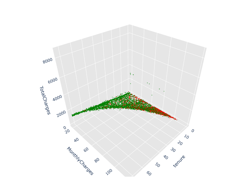
Figure 1: The relationship between Tenure, Monthly Charges, and Total Charges (Photo/Picture credit: Original).
2.2. Feature Engineering
This part is feature engineering. According to the article, the author Makashir points out that Feature Engineering techniques are typically applied after gathering and cleaning the input data [5]. Before doing feature engineering, it is important to create the variables and features. Then, add the ratio variables, the purpose is to calculate the ratio between the monthly charges and tenure, Total Charges, Non-protection, and other fields. After that, adding the log of the numeric field and adding statistical features. Then, plot the table and the table changes to analyze by 0 and 1 for binary code. Then, the next step is to use the target encoding & One-Hot encoding.
2.3. Target Encoding & One-Hot Encoding
Target encoding is a method used in machine learning to transform categorical data and target encoding substitutes the average target value of each category’s data points for a categorical feature. Before starting to do the encoding, the data does not need to be split and treated differently until doing the feature selection. However, when doing the target encoding, the target variable values in the train set should be used. Let's first find the train size and test size. After running the code, the answer is that the train size is 5634, and test size is 1409. The step is to divide two groups and start to do the Target encoding. First, pair all categorical features with other categorical features. After changing categorical variables with only two categories to dummy variables, the next step is to start to use the target encoding with a smoothing method and split the data into train test sets to perform target encoding.
The next method is One-Hot encoding. We use this categorical data encoding when the categorical feature is nominal. In one-hot encoding, for each level of a categorical feature, it creates a new variable, and each category is mapped with a binary variable containing either 0 or 1 [6]. It is a good way to use binary classification to analyze the data. The target encoding and the one-hot encoding are useful ways to do feature engineering. Their purpose is to transform the categorical data into a numerical format. Lastly, after running the code, the results are two matrices X and showing that the one-hot encoded matrix size is 7043 rows and 32 columns, and the target encoded matrix size is 7043 and 21 columns. So, these two methods get different sizes for two matrices.
3. Feature Selection
In this part, the main idea is calculating the KS and Churn Detection Rate then, using feature selection to analyze the data. First, the CDR, the Churn Detection Rate is almost 0.3, slightly larger than the average churn rate of 0.265. Next, the step is to do the univariate filter. The univariate filter is to analyze the rank of a single feature. Then, perform a split test on the encoded data and use the univariate filter to find features selected by the filter and now the target testing changes to 1409 rows and 18 columns. For one-hot testing, it changed to 1409 rows and 23 columns. This is the answer after analysis. After doing the filter method, the next is to do the wrapper method. These techniques evaluate subsets of features based on how well they perform with the chosen ML algorithms. The reason to use a wrapper method is to find the stepwise selection for target encoded data and use a graph to show the Stepwise Selection. The machine learning algorithm is the LGBM Classifier. The final performance is closer to 0.8 in Figure 2 and Figure 3.
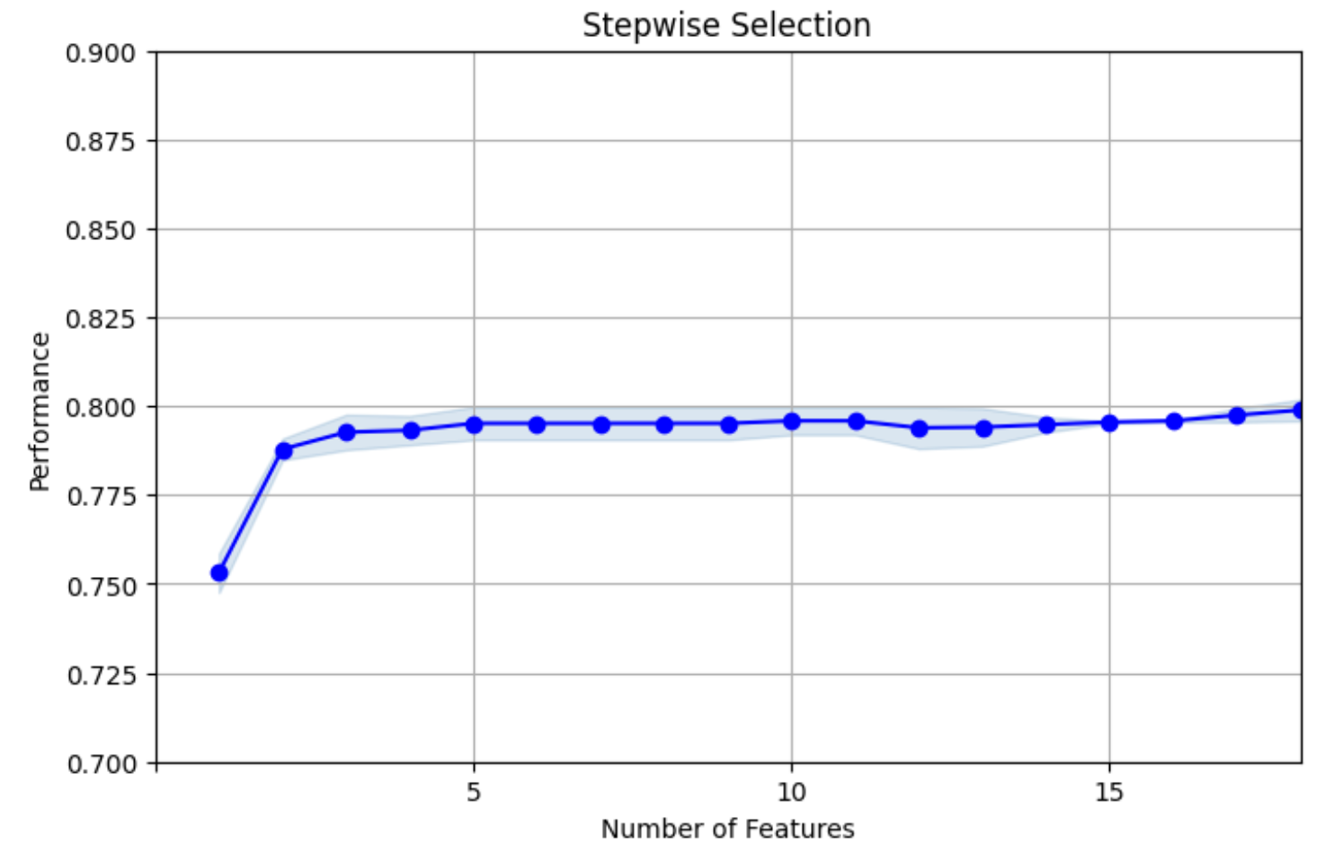
Figure 2: Stepwise Selection for Target encoded data (Photo/Picture credit: Original).
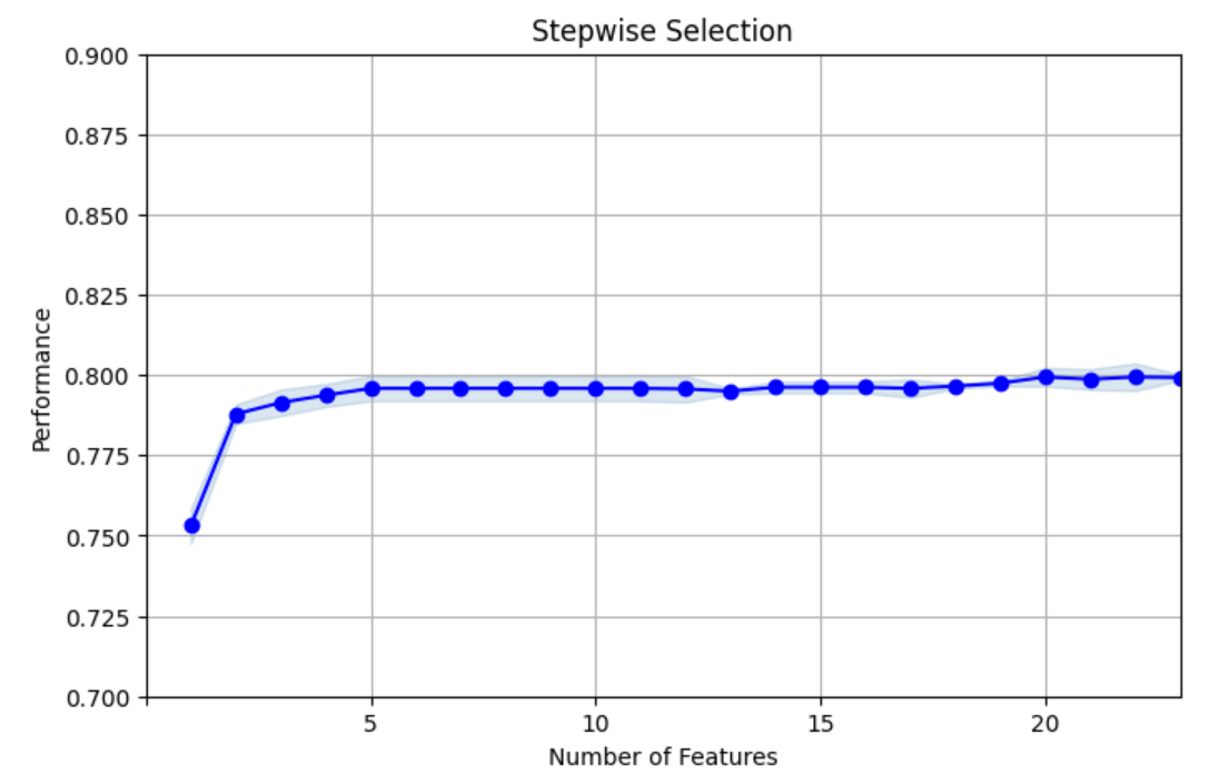
Figure 3: Stepwise Selection for One-Hot encoded data (Photo/Picture credit: Original).
For one-hot encoded data, the final performance is also closer to 0.8 but the number of features is more. Lastly, prepare the final features to be used for Model Building for target encoded variables and one-hot encoded variables. The final train X shape for the target encoded is 5634 rows and 5 columns, final test X shape for the target encoded is 1409 rows and 5 columns. The final train X shape for one-hot encoded is 5634 rows and 5 columns, and the final test X shape for one-hot encoded is 1409 rows and 5 columns. The final train y shape is 5634 rows and 1 column, the final test y shape is 1409 rows and 1 column.
4. Model Tuning
4.1. Four Models: LR, Gradient Boosting Tree (GBT), Random Forest (RF), Neural Network (NN)
The model Tuning part, mostly talked about what each model is, how these models work, and finding the optimal parameter combination based on the specified score type. First, let’s talk about LR. Binary, multinomial, and ordinal LR are all possible [7]. First, let’s discuss binary LR. The LR predicts that the input class belongs to class 0 based on the real-valued inputs. The output is classified as class 0 if the forecast is greater than 0.5, and class 1 otherwise [7]. This method is a good way to change the binary code and it becomes easy to classify the data. The second method is called the GBT. By using models to calculate the error as residuals of previously applied models, gradient boosting showed a methodology that combines the two to provide the final forecast [8]. Another method is RF. A group of randomized decision trees (DTs) is called a RF. A model in the shape of a tree structure is established via DT, a non-parametric machine learning technique. Until there is just one record left in the subset, DT repeatedly splits the provided data into progressively smaller subgroups [9]. The previous saying showed that the step of RF classifier and choose the best value at the end of the algorithm. The last method is the NN or Artificial NN (ANN). The signaling behavior of neurons in biological NNs serves as an inspiration for artificial NNs. To forecast an outcome, artificial NNs, which are made up of a population of neurons connected by intricate signaling pathways, use this structure to assess intricate relationships between a set of observable covariates [10]. These four methods are different and their algorithm showed different results for advantages and disadvantages. The following figure 4 shows the results for these four models.
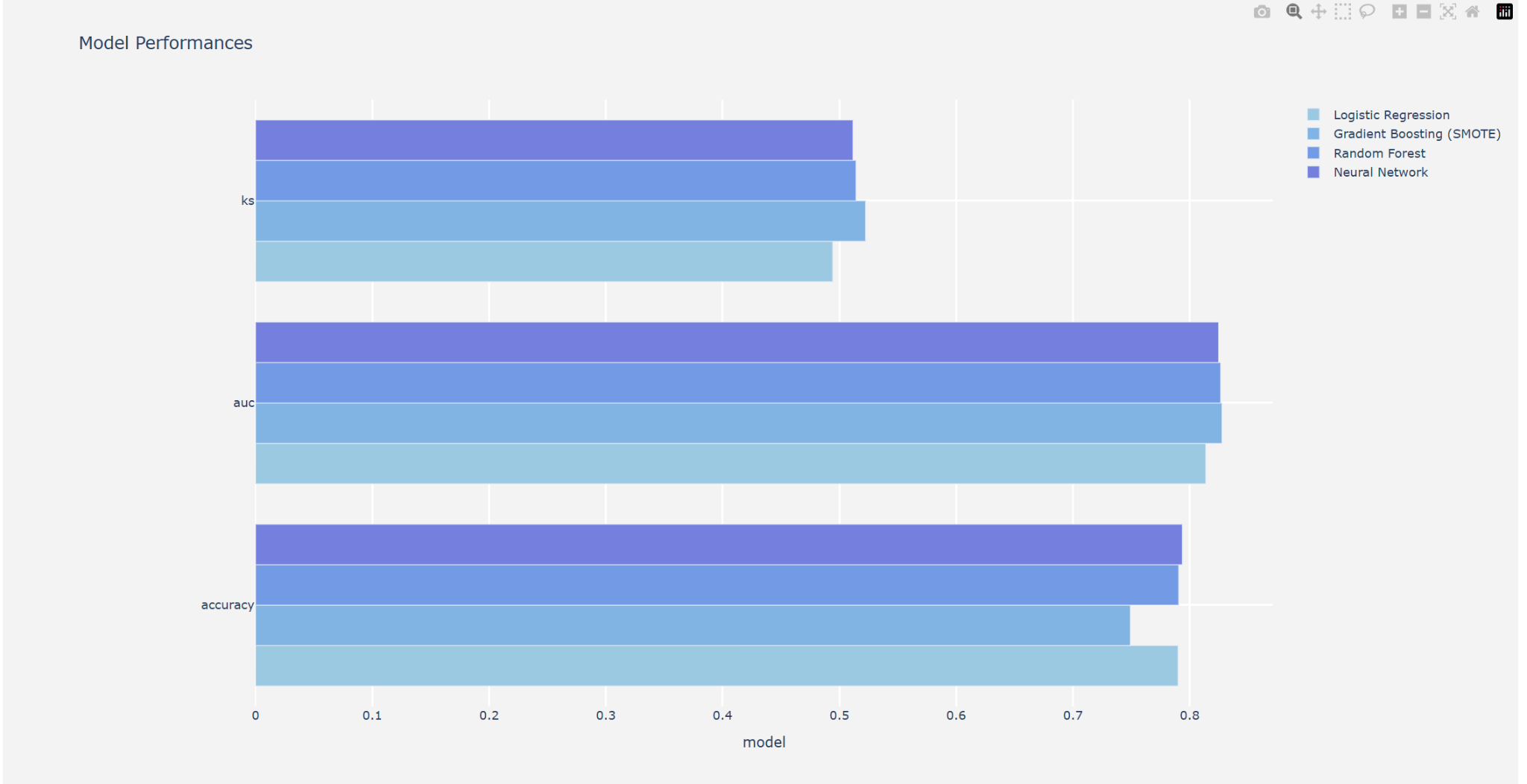
Figure 4: The data for KS, AUC, and accuracy calculated by Four models (Photo/Picture credit: Original).
4.2. Stacking Model & Final Analysis, Final Results
Let’s talk about the Stacking Model. In machine learning, stacking is a powerful ensemble learning technique that aggregates the predictions of multiple base models to get a final prediction with improved performance [11]. After building the model, then, choose a good model and get the final results. From figure 5, it concludes that the performance scores on the hold-out set are only slightly inferior than the cross-validation scores on the training set. That means the models don’t overfit. Finally, the performance of the four models is very close to each other. The following picture shows that the LR with the upsampling method is better.
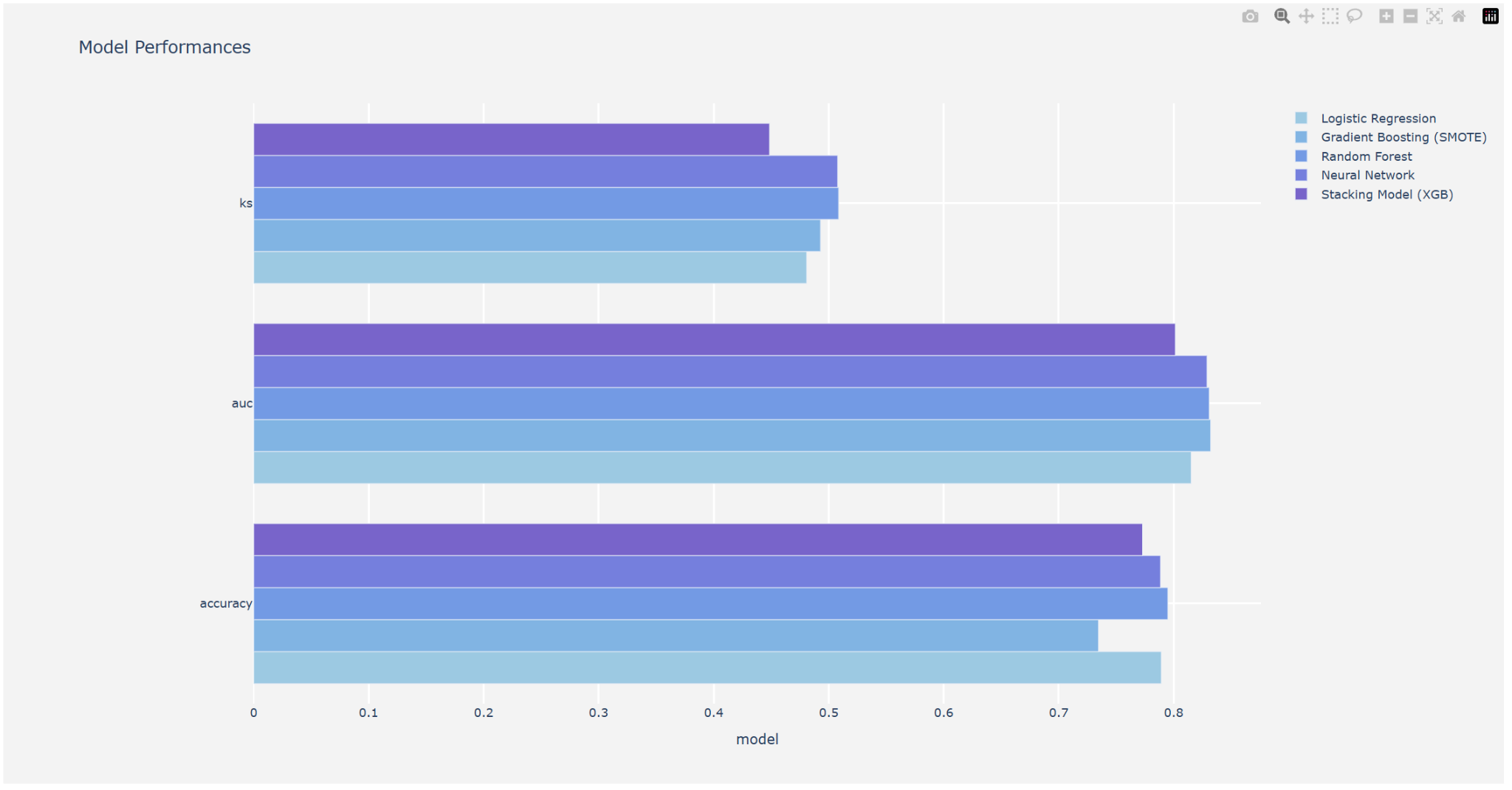
Figure 5: Model performance on the hold-out set (Photo/Picture credit: Original).
5. Discussion
From the previous results, it concluded that the LR with the upsampling method is better. In the study, the LR model performed significantly better than other models on computation and interpretability, indicating its good adaptability in predicting the customer attrition rate. This is consistent with the results in Prakathi [12]. The data may not demonstrate a complex relationship between the predictor factors and the target variable, which is why the RF Model and other models perform poorly. This implies that the decision tree model would have trouble enhancing its predictive accuracy if the data in our situation is somewhat simple or lacks complex patterns. However, because the algorithms can accurately capture the linear elements of the data and generate attrition predictions, the LR did better. The shortcoming of the study mainly lies in the data set because of the sensitive nature of banking data, people cannot access more datasets. In view of the above shortcoming, future research can consider expanding the datasets. Getting more datasets can enhance the generalizability of predictions. Another improvement is to use additional prediction algorithms. Finally, we can find more results and compare more models to analyze why these models are useful or not. In addition, different prediction algorithms are suitable for different customer brackets and lead to more impact predictions. This improvement can have a practical application value of the model and understand how to predict the customer attrition rate.
6. Conclusion
The customer churn rate is a serious problem. People started to do the data analysis for the customer churn and understand what’s customer churn rate is and how to solve the business problem. The business problem is to know what the customer churn rate is and win back defecting clients. Then, many people started to do the data analysis and try to solve the business problem. First, do exploratory data analysis. This part showed how to evaluate the customer attrition, and their variable distributions and plot the graph. After the exploratory data analysis, the next part is about feature engineering. It included the Target Encoding & One-Hot Encoding. The purpose of encoding can use binary classification and it looks clearly after grouping the data. The next step is to get the correlation matrix and look at the table about variable summary. Now, let’s try to analyze by using feature selection. It included the univariate filter and stepwise selection wrapper method. The wrapper method evaluates subsets of features based on how well they perform with the chosen ML algorithms and finds the final features to be used for model building. That means in the Model building part, the purpose is to build the model and find which features are better. In this part, these several models are needed to be used. For example, LR, Decision Tree, RF, Gradient Boosting, and so on. After evaluating these models, the results concluded that these models are a good fit for the model, there is not much difference between the Target Encoded Features and One-Hot Encoded Features for the data set. So, from the data and the model performance, they conclude that the gradient-boosted tree, LR, and NN are the top 3 models for the data sets. Now, the next process is the model tuning. Four models should be used: LR, GBT, RF, and NN. After running the code, the algorithm shows the table by using these four models and their results are close, it also shows that the dataset is suitable and the dataset performs very well. The final step is to add a stacking model and analyze it again. After running the code, the results showed that the model does not overfit. In summary, these four models results are very close but the LR Model with upsampling method is better. These four models, it showed each result that predicted the customer churn rate. Since customer churn becomes a serious problem, it is important to use models to analyze why there exists customer churn, how can reduce the churn, and how to predict the customer churn rate. These four models will become helpful in the future and help people improve their knowledge about customer churn.