


1. Introduction
In modern power distribution systems, particularly in 110kV networks, the swift and precise identification of fault locations is crucial for maintaining reliability and minimizing disruptions. It can reduce downtime and enhance the operational reliability of the power supply system. Modern electrical grids are now becoming increasingly integrated with advanced monitoring and control systems. So, the demand for an accurate and stable fault detection method grows [1].
Faults can be caused by various reasons, including weather events, equipment failures, and human error, leading to economic losses and safety hazards. Traditional techniques, such as impedance-based methods, often need more accuracy due to challenges posed by complex network topologies, variable load conditions, and electrical noise [2]. Another traditional method is manual line patrol. This method can be used to detect faults in the distribution lines and offers high accuracy. However, it has significant labor and time costs [3].
The method for finding wave faults accurately helps to make operations more efficient and also increases the reliability of the power supply overall. This paper aims to explore a new implementation of the method within 110kV distribution networks for the high voltage power transmission tower, exploring its effectiveness in enhancing fault management processes and paving the way for future advancements in electrical infrastructure.
To surpass the constraints of the traditional methods, the new accuracy wave fault location method should have the following functions. For example, the method should gather the wave information, detect the fault location, and upload the location data quickly. Although Traditional computers can be programmed to detect and upload the fault location easily, they cannot handle waveform signals at a frequency of 25 MHz. So, a high-speed FPGA is required for the implementation of the wave fault location method. When faults on the distribution lines occur, FPGA can analyze the current waveforms, which are captured from the power lines through current transformers and Analog to Digital Converter (ADC). With their parallel processing capabilities, FPGAs facilitate real-time analysis, making it possible to implement complex algorithms swiftly and efficiently. FPGA can calculate the fault location with the help of an accurate time system. After finding the fault location, FPGA can build a UART to upload the fault location data and waveforms to the computers.
2. Basic concepts of the wave fault location method
In power lines, traveling wave distance measurement is used to locate faults quickly. Typical faults include ungrounding, small resistance grounding, and arc suppression coil grounding. Signals can reflect strongly at the termination when ungrounded, causing waveform distortions. Compared with the ungrounded, small resistance grounding can effectively minimize the reflections. It gives the signal a steady reference and cuts down on distortion. ASC grounding changes how short waves act, making the wave shape smoother with less distortion [4].
When a disturbance occurs in the distribution lines, the current signals and voltage signals will change suddenly, which creates waves that travel along the line. These waves are called traveling waves. When these waves reach different monitoring points, the fault location can be calculated using the wave propagation speed and the time information. The wave propagation speed depends on the material of the power line.
There are two main ways to get the exact fault location, which are called single-ended and double-ended wave fault location method [5, 6]. In the single-ended fault location method, one monitoring equipment is put at only one end of the line. This way, the distance from that monitoring device to the fault location can be calculated, as seen in Figure 1 [7, 8].
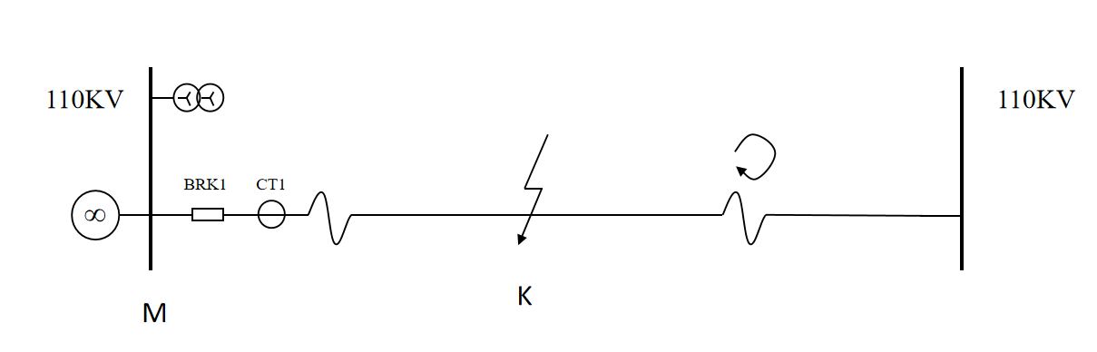
Figure 1: Single-ended wave fault location method
The fault location for the single-ended wave fault location method on the distribution lines is calculated through the following formula.
\( {D_{MK}} = \frac{1}{2}v∆t \) (1)
Where \( {D_{MK}} \) means the distance between the monitoring equipment and the fault location on the distribution line, v represents the wave propagation velocity and \( ∆t \) represents the time difference between the first arriving traveling wave signal and the following reflected wave signal.
In the double-ended wave fault location method, two monitoring equipment are installed at both ends of the distribution lines. The fault location can be calculated by calculating the time difference of the first traveling wave arriving at both monitoring points. As shown in Figure 2, the wave generated by the disturbance propagates to endpoints of the distribution line, M and N. Two traveling wave monitoring devices are installed at M and N [9].
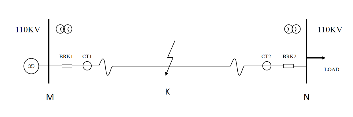
Figure 2: Double-ended wave fault location method
The fault location for the double-ended wave fault location method can be calculated through the following formula.
\( {D_{MK}} = \frac{1}{2}(v({T_{M}}-{T_{N}})+L) \) (2)
Where DMK means the distance from the monitoring equipment M to the fault location K. TM and TN represent the times at which the first traveling wave reaches devices M and N. The length of the distribution line between position M and N is L. And v represents the propagation speed of the wave in the distribution lines.
3. Wave fault location method based on FPGA
The exact fault location is calculated using an FPGA board, which can easily sample, detect, and locate faults by analyzing waveforms generated from disturbances. When a disturbance in the distribution lines occurs, the fault produces traveling waves that the FPGA can capture using current transformers and ADC. These signals will be processed in FPGA. FPGA can execute complex algorithms rapidly. The method includes establishing a time system, signal filtering method, waveform analysis method, and the calculation of the fault location.
3.1. Time system in FPGA
The stable and accurate time system is a ranging technology designed to improve measurement precision and system reliability. It can be used to calculate the distance by real-time monitoring of the propagation time of traveling waves. This chapter will show a stable and accurate time system based on FPGA.
The stable and accurate time system is based on a Global Positioning System (GPS) chip and an adjustment algorithm. GPS chips provide PPS (Pulse Per Second) signals based on the GPS's time synchronization characteristics. Satellites generate time signals using highly accurate atomic clocks, which are broadcast to ground receivers. The receiver can get precise time information upon receiving signals from multiple satellites. The rising edge of this signal represents a standard time mark at each whole second. It can be used to adjust the timing system of FPGA and synchronize the time between different monitoring devices [10].
Due to the blockage of GPS signals, GPS cannot provide a standard time mark at this moment. The synchronization between different monitoring devices will fail, leading to the wrong fault location being calculated. FPGA should build a timing system to avoid this problem. It is based on the crystal oscillator and the PPS signal. The crystal oscillator should be as stable and accurate as possible, usually a TCXO. A stable and accurate timing system can be generated as follows:
• First, FPGA is used to build a counter that counts the period of the PPS signal, aided by a crystal oscillator that can provide a clock signal with a frequency of 100MHz.
• Calculate the average of the previous 60 counter results.
• Suppose the new result is larger than the average, add the average by one. If the new result is smaller, the average will be decreased by one. If the new result equals the average, the average remains unchanged.
• If the PPS signal is lost, use the calculated average value as the period for that second. Otherwise, continue with step 1.
FPGA can build a time system that provides each sampled point with a precise time. This guarantees the precision of the distance measurement.
3.2. Discrete Wavelet Transform
Discrete Fourier Transform (DFT) is a mathematical approach to analyze the frequency parts of discrete signals. A series of samples in the time domain are transformed into the coefficients in the frequency domain. While the DFT effectively reveals the presence of fixed frequency components, it loses time information, which is crucial for calculating fault locations. Therefore, another mathematical technique, which is called the Discrete Wavelet Transform (DWT), should be calculated to get not only the frequency components and the time information [11].
Compared to DFT, DWT gives both time and frequency information, helping to analyze short-term or changing signals more closely. DWT can be used to analyze signals at different levels of detail. This is really helpful for seeing both high-frequency parts and low-frequency patterns at the same time.
The DWT is a powerful mathematical tool in signal processing. The tool is effective for analyzing signals across various scales. It changes a signal into wavelet coefficients that show both frequency and time details. The DWT does this by breaking down the signal into different frequency parts using filters, which is called signal decomposition. After the decomposition, the resulting approximation and detail coefficients need to be down-sampled by a factor of 2. The mathematical representation of the DWT is shown as follows:
\( {A_{i}}[n] = \sum _{m}h[m]x[n-2m] \)
\( {D_{i}}[n] = \sum _{m}g[m]x[n-2m] \)
Where the approximation coefficients at level i are represented by Ai[n], the detail coefficients at level i are represented by Di[n], h[m] are the low-pass filter coefficients, and g[m] are the high-pass filter coefficients. The coefficients of these two filters depend on the wavelet basis function which is used. Signal x[n] can be represented as the input signal, approximation, or detail coefficients.
DWT can be computed for multiple layers by recursive decomposition. A specific frequency range can be represented in a multilevel wavelet transform. For instance, the frequency range of [0, Fs/4] is represented by first-level approximation coefficients, and the frequency range of [Fs/4, Fs/2] is represented by first-level detail coefficients, where Fs represents the sampling frequency. The frequency range of [0, Fs/8] is represented by the second-level approximation coefficients, and the frequency range of [Fs/8, Fs/4] is shown by the second-level detail coefficients.
Inverse Discrete Wavelet Transform (IDWT) is a mathematical operation. This operation is used to reconstruct the original signal from its wavelet coefficients. The calculation of the IDWT should be started by up-sampling the coefficients with zeros by a factor of 2 first. After the up-sampling process, the coefficients are calculated through the high-pass or low-pass reconstruction filters like DWT. The outputs of these reconstruction filters are then added together to obtain the reconstructed signal. IDWT can also be computed for multiple layers by recursive decomposition. By calculating IDWT across multiple layers, the wave with a specific frequency range can be gotten from the input signal.
3.3. Signal filtering
If the fundamental wave of the input signal needs to be removed from the signal, DFT should be used to calculate the frequency of the fundamental wave first. After the calculation of the frequency of the fundamental wave, it can be filtered through the high pass circuit on the FPGA board.
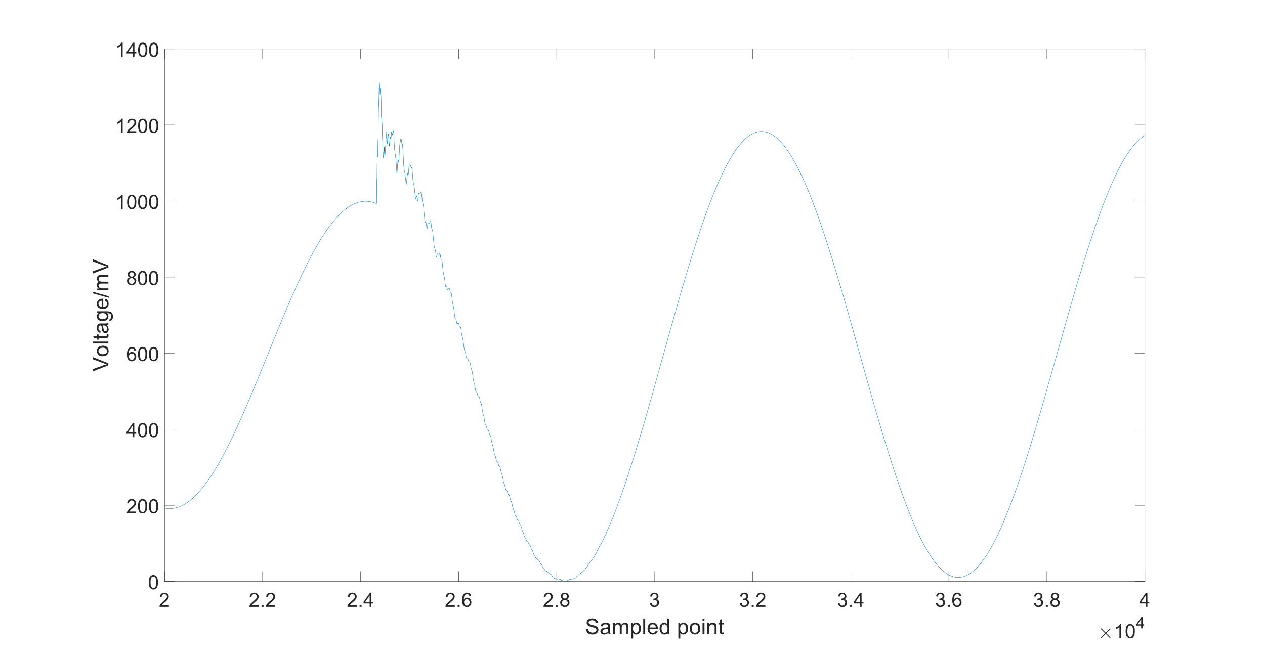
Figure 3: Input signal with the traveling wave which is sampled by the ADC
Figure 3 shows an input signal with a traveling wave and the fundamental wave. The frequency range of the traveling wave should be from 0 to infinity [5]. The frequency of the fundamental wave is about 50 Hz. The result of the calculation of the DFT is shown in Figure 4.
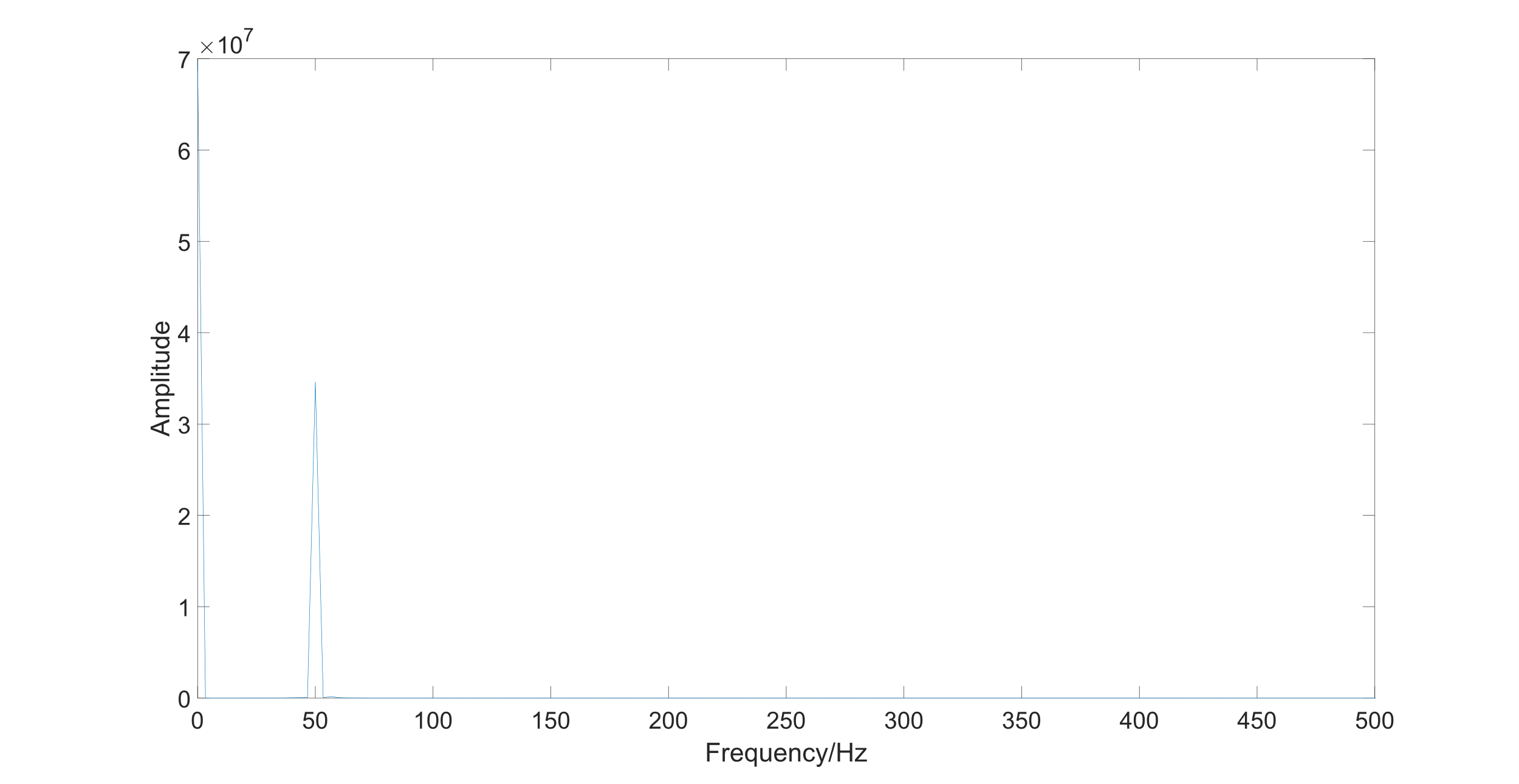
Figure 4: DFT result of the signal from the power line with traveling wave
When the cut-off frequency of the high pass filter is set to 200Hz, fundamental wave in the input signal will be filtered. After filtering the fundamental wave, it is essential to remove noise from the signal through multiple layers of Inverse Discrete Wavelet Transform (IDWT) for effective wavefront detection [11]. The steps to remove the noise are as follows:
• Calculate the IDWT for a signal that does not contain a traveling wave.
• Determine the maximum absolute value from the IDWT results. This value will serve as the noise threshold and be set in the FPGA.
• For a signal with a traveling wave, if the IDWT value at a specific point is lower than the threshold, classify that signal as noise. If the value exceeds the threshold, classify it as a valid signal.
3.4. Wavefront detection
After removing the fundamental wave and noises from the signal, the FPGA should compute the DWT and IDWT using the data provided by the ADC on the FPGA board. When a traveling wave is generated on the distribution lines, it induces an instantaneous change in the wave profile, with the wavefront representing the first change point on the signal [4].
To effectively identify this first change-point, the DWT of the signal should be calculated across three layers. For the detail coefficients of the first layer, find the first point i, which d[i] fulfills the following conditions:
\( |d[i]| \gt d[i±1]+2 \gt d[i±2]+2 \) (3)
For point i, the detail coefficients of the second and third layers should be larger than the noise threshold for their corresponding layer.
The first change point which fulfills these conditions is taken as the wavefront of the traveling wave. The time information of point i is given by the time system of the FPGA.
3.5. Distance measurement
The exact fault location of in the 110KV distribution line can be calculated through the following formula.
\( {D_{MK}} = \frac{1}{2}(v({T_{M}}-{T_{N}})+L) \) (4)
The wave speed of traveling waves is related to the characteristics of the line itself, which contain the inductance and capacitance per unit length of the line. The wave propagation speed of traveling waves in a distribution line is determined solely by the properties of its insulating medium, independent of the conductor's material and cross-sectional area. For example, the wave speed in overhead lines is 294 km/ms, in paper-insulated cable lines, it is 160 km/ms, and in cross-linked polyethylene cables, it is 170 km/ms. In a 110kV distribution network, the wave speed is 294 km/ms. So, the distance between device M and the error location can be calculated if the time difference is known.
4. Benchmark
In this chapter, the accuracy and stability of the time system will be tested first. The double-ended wave fault location method is used to find the exact fault location on the power line next. In order to get the input signal of the FPGA board, two different kinds of current transformers are used. They gather the current signal of the power line and then send a current signal to the FPGA board. The current will be transferred into a voltage signal by using a sampling resistor and then transferred to the ADC. The sampling rate of the ADC is 25MHz. FPGA reads the data in ADC and calculates the exact fault location. The location information will be transferred to the PC by using UART. Finally, the results will be shown in MATLAB. Figure 5 shows the frequency of the TXCO. The frequency colored by blue varies from 99999895Hz to 99999899Hz in 500 seconds. The time system generated by the FPGA is colored orange.
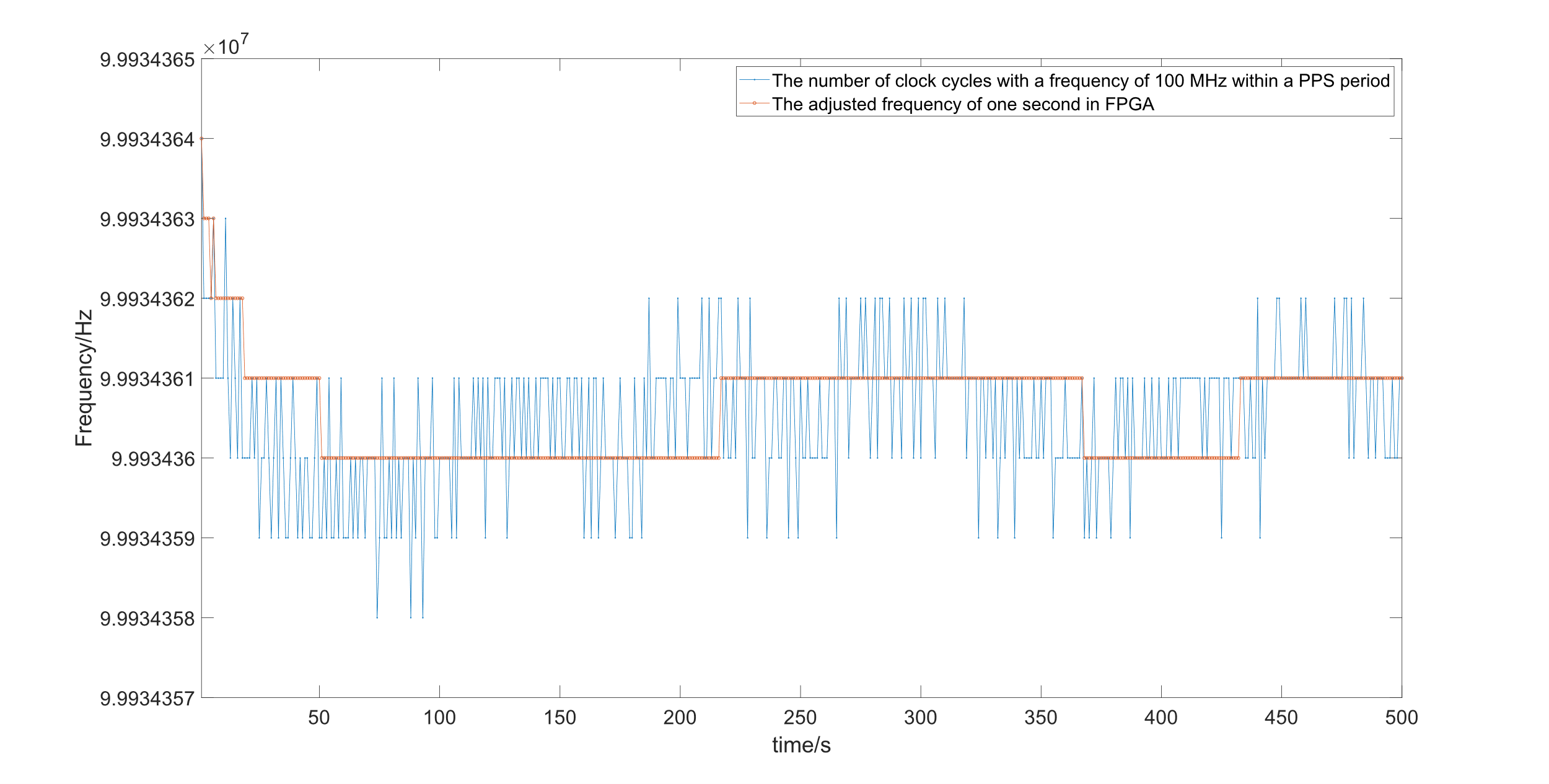
Figure 5: Frequency of the TXCO which is counted by the clock signal in FPGA
The threshold of the time difference between the time of the FPGA time system and real-time is set to 100ns. The hold time is defined as the time length between the time when GPS lost the PPS signal and the time difference reached the threshold value.
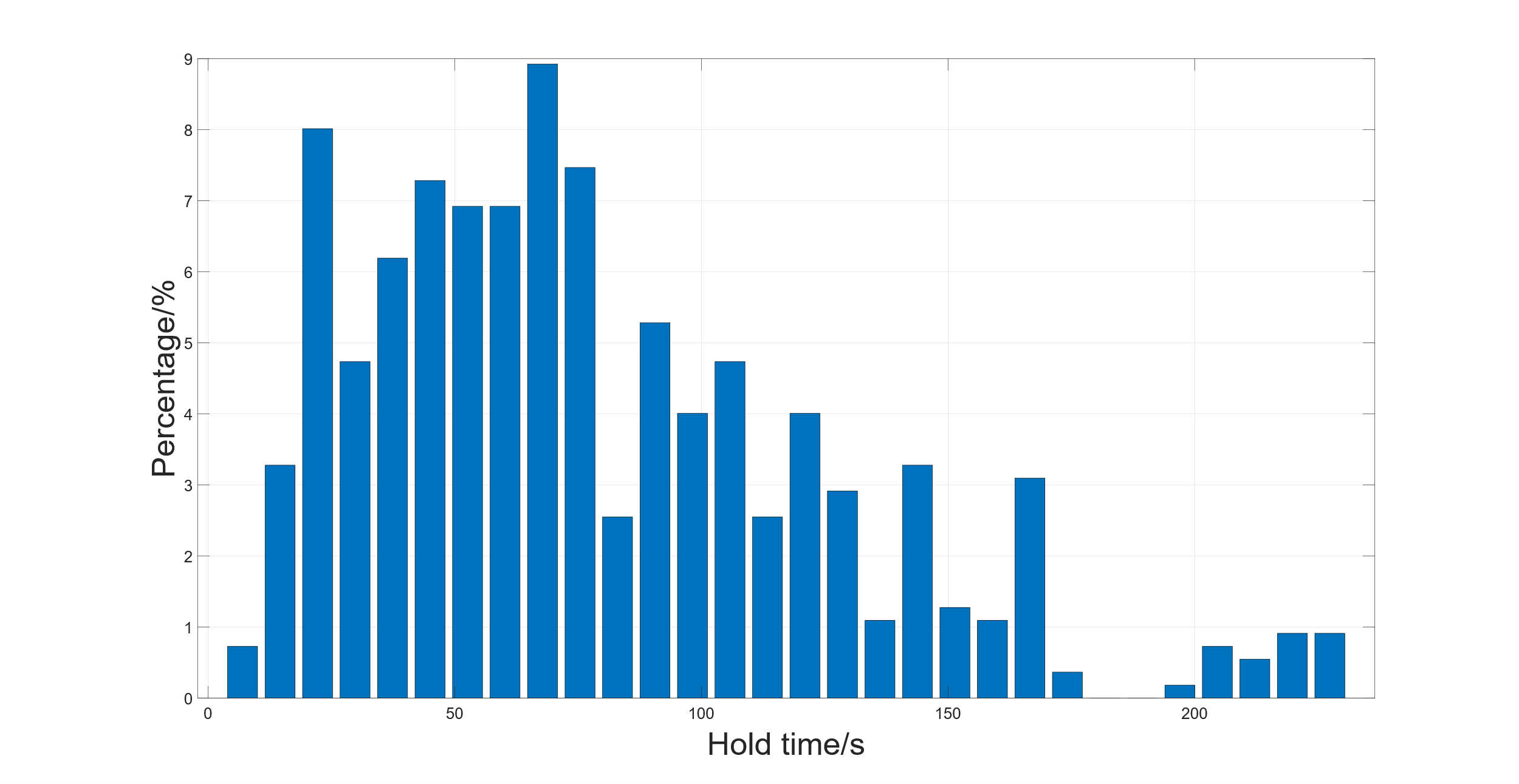
Figure 6: Hold time for the time when GPS lost the PPS signal
Figure 6 shows the frequency distribution histogram for the hold time in 500 seconds. The X-axis represents the hold time for each second. The Y-axis represents the frequency of the observations. The average hold time is 82 seconds. Moreover, the worst hold time is 17 seconds, and the best hold time is 235 seconds. After testing several TXCOs on the FPGA board, the best and worst hold times greatly depend on the stability of the TXCOs. A higher stability of the TXCO guarantees a better hold time for the time system.
The distance between the two monitoring devices is 10 km. The wavelet function is Daubechies 4 wavelet. The fault is triggered by the Earth (ground) fault arc suppression coils. Furthermore, Phase B is the problem phase. The sampled three-phase voltage signal with the traveling wave signal in the distribution line is shown in Figure 7. The figure shows the signal of phases A, B, and C from top to bottom. The sampling rate of the ADC is 400KHz.
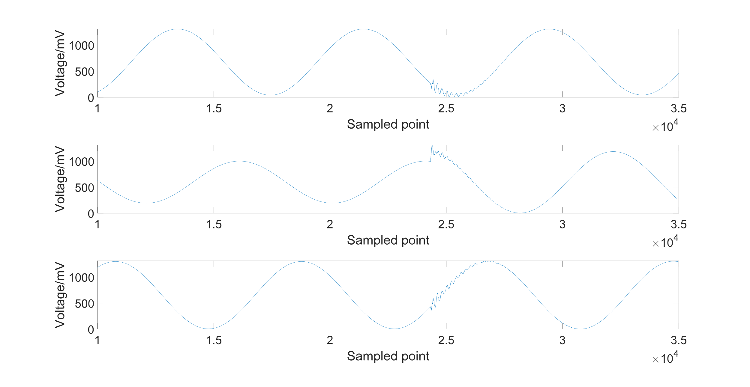
Figure 7: Input signals are gathered by ADC from monitoring device M
The disturbances are more noticeable and have larger amplitudes on the fault phase usually. This makes it easier to analyze and locate the fault location in the following steps. As a result, all further calculations are centered around the fault phase B.
The wave in phase B should be used to calculate the DWT and IDWT in order to get the noise value and the exact fault location. As is shown in Figure 7, the peak-to-peak voltage of the original signal of phase B is about 1300 mVpp. The traveling wave signal of phase B after passing through the high pass filter is shown in Figure 8. The cut-off frequency of the high pass filter is set to 200 Hz.
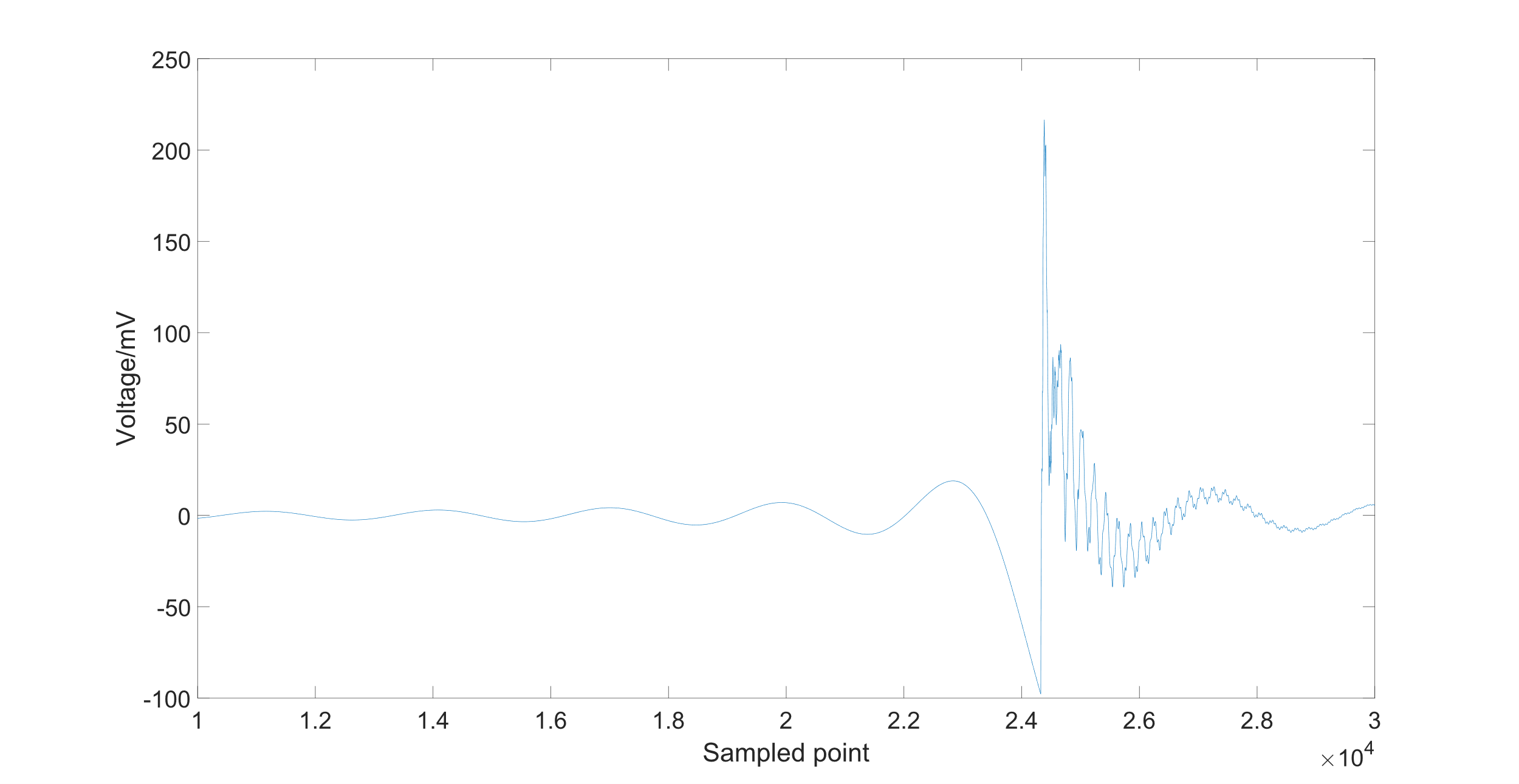
Figure 8: The wave signal after passing through the high pass filter for monitor device M
After the filtering, calculate the DWT and IDWT for the noise of Phase B when there is no traveling wave. The wave signal and the result of the detail coefficients for the first three layers are shown in Figure 9.
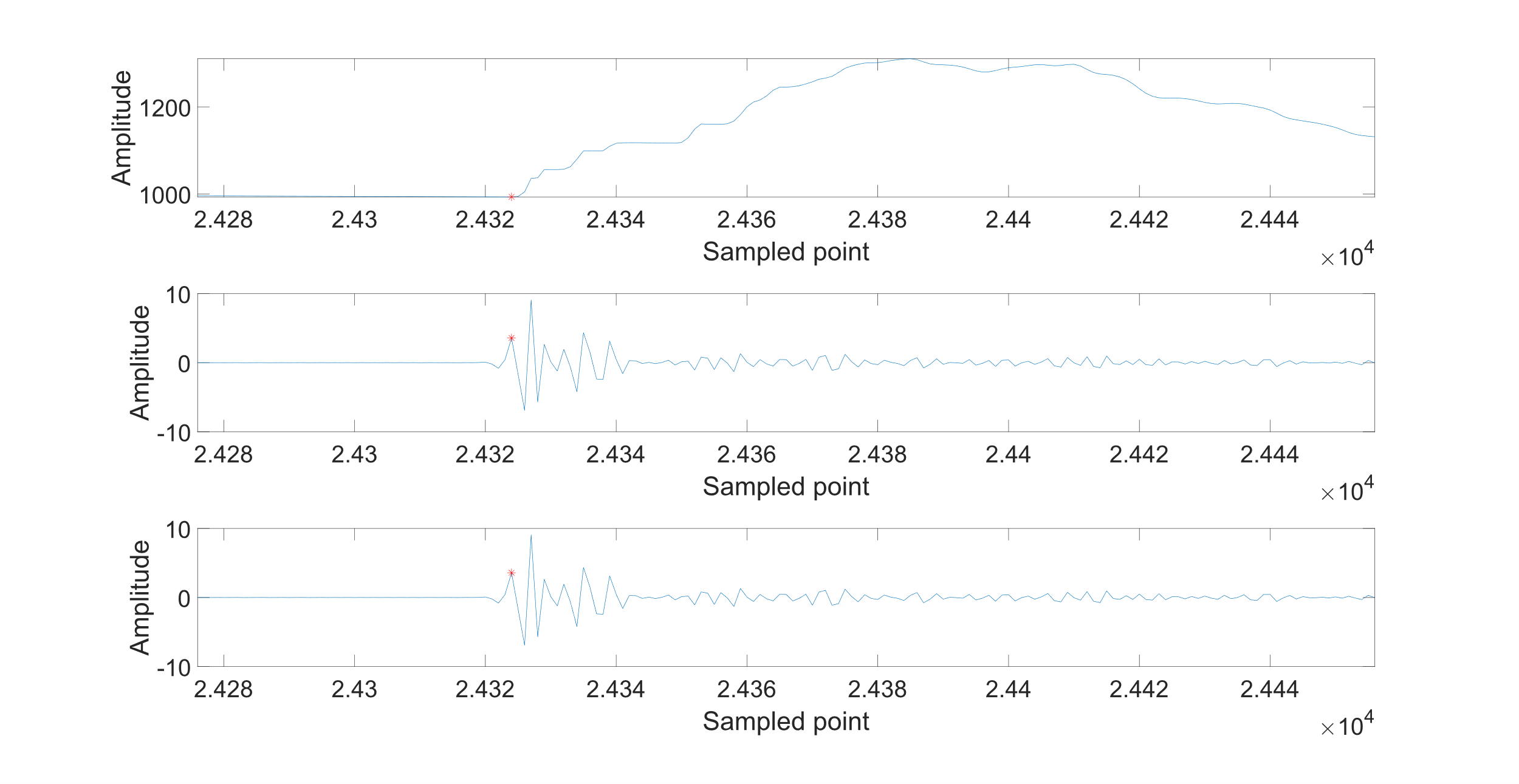
Figure 9: Wave signal of Phase B and the first two layers of IDWT
According to Figure 9, the noise for the first three layers of IDWT is all 0.01026 mV. The fault location is 24322. The error between the actual fault location and the calculated fault location is 2 points.
The original three-phase traveling wave in the distribution line for another monitoring device is shown in Figure 10. The traveling wave signal of phase B passes through the high pass filter with a cut-off frequency of 200Hz.
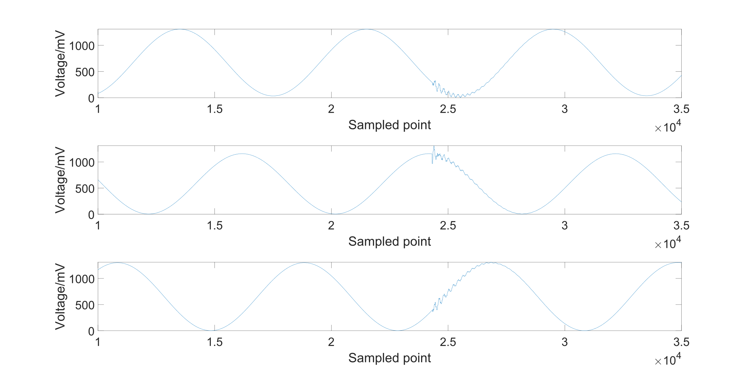
Figure 10: The wave signal after passing through the high pass filter for monitor device M
After the filtering fundamental wave, calculate the DWT and IDWT for the noise of Phase B when there is no disturbance in the power lines. The wave signal and the result of the detail coefficients for the first three layers are shown in Figure 11.
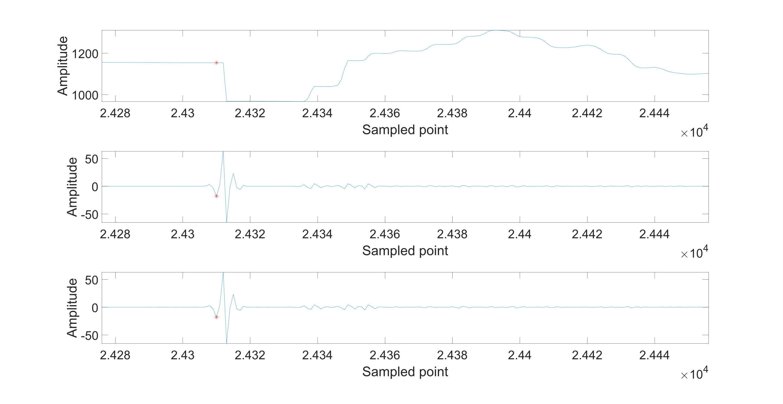
Figure 11: Wave signal of Phase B and the first two layers of IDWT for monitor device M
According to Figure 11, the noise for the first three layers of IDWT are all 0.5129 mV. The exact location of the disturbance on the distribution line for phase B is 24308. The error between the actual fault location and the calculated location is also 2 points. So, the time difference between the traveling waves arriving at the two monitoring devices can be calculated, and it is 140 nanoseconds.
So, by applying the data in the formula below, the distance between monitoring device M and the fault location K is DMK, which is about 5084 meters.
\( {D_{MK}}=\frac{1}{2}(V({T_{M}}-{T_{N}})+L) \) (5)
5. Conclusion
This paper reviews the current wave fault location methods in 110kV distribution networks and presents a new accurate method based on FPGA. It can help to detect fault locations with the newly introduced method in the distribution lines. In the method, a stable and accurate time system is contained, which has an accuracy of 10 nanoseconds. If the GPS core on the FPGA board loses the signal from the satellite, the time system can be stable for at least 17 seconds. The traveling wave localization error is about 30 meters due to the ADC error on the FPGA board. It enhances fault detection significantly. The new method also makes use of the advantages of FPGA, which can help analyze voltage waveforms in real time, provide accurate location results, and react quickly. Not only can operational efficiencies be improved, but the downtime of the power system can also be reduced by implementing the new fault location method.
However, the new method is limited only to high-voltage transmission towers, in which the power lines are almost straight. When the lines are buried underground, it may not be suitable because the line may not be straight. After the calculation of the fault location, manual line patrol is still needed because the accuracy is still not enough. Future studies should focus on developing more robust algorithms and testing their scalability across different voltage levels and network configurations, such as 10KV and 550KV distribution networks. It should also be able to detect and find the accurate fault location when the power lines are coiled several times in some places. Additionally, using machine learning techniques is also an option. AI can be trained to detect the fault location quickly and accurately through machine learning technologies. These technologies can ensure a stable energy supply for future generations.