Aerodynamic Characteristics of NACA 0018 Based on CFD Method at Low Reynolds Number

1. Introduction

Small fixed-wing UAV (Unmanned Aerial Vehicle) have become an important branch of modern aviation due to their efficient and stable flight and long endurance capabilities [1]. The UAVs are widely used in monitoring ecosystems, such as wetlands, border patrols, disaster assessment, and topographic mapping [2,3]. The airfoils have a decisive influence on the aerodynamic properties of fixed-wing UAVs, especially the coefficients of lift and drag [4].

In recent years, the study of aerodynamic properties of airfoils has gradually become an important topic in the field of aerospace. Researchers have used a variety of advanced technologies, such as numerical simulation, experimental flow field test and wind tunnel test, to explore the aerodynamic properties of different airfoils [5-7]. The research of Johnson et al. shows that the lift of the NACA 0012 airfoil maintains good characteristics at high Reynolds numbers and angles of attack [8]. The aerodynamic properties of the NACA 0012 airfoil can be significantly improved by detailed geometric optimization. Brunner et al. used a high-pressure wind tunnel to study the aerodynamics of NACA 0021 at high Reynolds numbers and found that once the Reynolds number rose above a certain point, the stall type changed slowly from the stall of the trailing edge to the stall of the leading edge, causing a fundamental alteration in the flow behaviour [9]. When the UAV is flying at low speed, the airfoils will face the problem of low Reynolds number flow. Low Reynolds number flow has a strong nonlinear effect and flow instability [10]. The traditional high Reynolds number flow theory is no longer applicable in this case.

With the development of CFD (Computational Fluid Dynamics), the aerodynamic properties of airfoils can be accurately predicted and analyzed by numerical simulation. Compared with traditional methods involving frequent parameter changes large experimental costs and time constraints, CFD technology has higher cost-effectiveness and time efficiency [11]. It can flexibly simulate airflow in various complex environments and provide detailed information on flow characteristics such as pressure distribution, velocity distribution and vortex structure. Thus, the use of CFD greatly shortens the research cycle and accelerates the optimization process of airfoil design.

Among numerous kinds of airfoils, the symmetrical airfoil NACA 0018 can produce more lift and maintain less drag at a lower angle of attack and Reynolds number [12]. Thus, through more optimized design and optimization, it is expected to further improve the flight efficiency of UAVs. Therefore, based on CFD simulation software—ANSYS Fluent, this paper systematically studies the aerodynamic properties of NACA 0018 at 3×10⁵≤Re (Reynolds number) ≤5×10⁵ and 0°≤AOA (angle of attack) ≤20°. The study can provide theoretical support for the development of low Reynolds number flow theory, as well as guide the optimization of low-speed flight performance of UAV.

2. Methodology

The simulation process begins with using SpaceClaim to create a geometric model, followed by meshing the model surface and fluid domain using Fluent Meshing. Then using ANSYS Fluent to define the boundary conditions and fluid solver parameters. Finally checking the convergence and performs post-processing.

2.1. Geometric model

This paper selects NACA 0018 as the research object, which is a symmetrical airfoil with a maximum thickness of 18% of the chord length. The geometric coordinates of the airfoil were imported into Fluent to create the geometric shape for CFD simulation. The geometric shape of the NACA 0018 is shown in Figure 1. Figure 2 shows the computational domain used for simulation. The inlet sections are both set with. The outlet of pressure is configured in the outlet section.

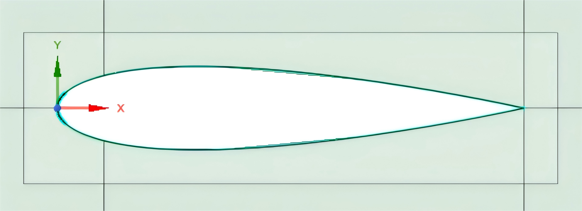
Figure 1: Geometric model

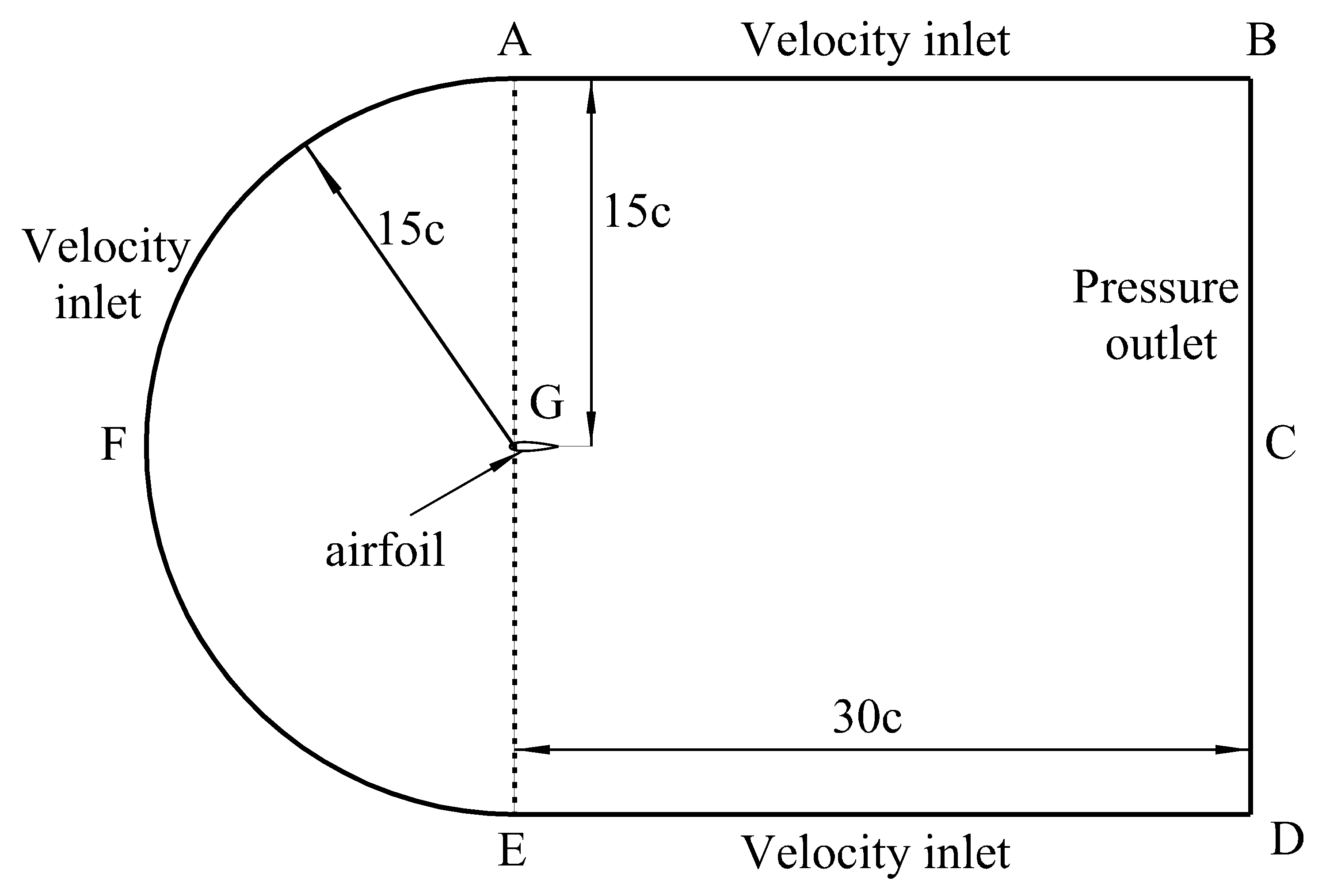
Figure 2: Computational domain

2.2. Grid

2.2.1. Grid meshing

The quality of mesh division directly affects the accuracy of numerical results. Therefore, this paper chooses a two-dimensional structured mesh to generate the mesh for the airfoil and computational domain. To better simulate the flow field movement, the computational domain is divided into a "C" type computational domain with six sub-domains to solve the equations in each domain segment. The external domain is meshed with coarser unit edge lengths to optimize computational efficiency and reduce computational costs. The airfoil area uses a fine mesh to better reflect the airflow movement. A bias factor is assigned to control the rate of change between mesh units. The mesh division at the computational domain is shown in Figure 3, and the local detail of the airfoil mesh is shown in Figure 4. The entire area has a total of 200,900 mesh units and 200,000 nodes.

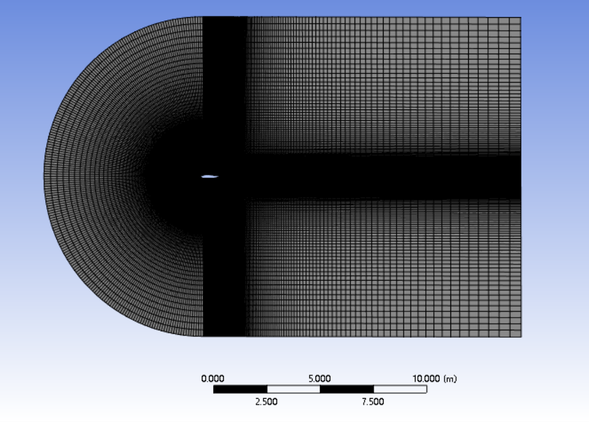
Figure 3: Computational domain grid

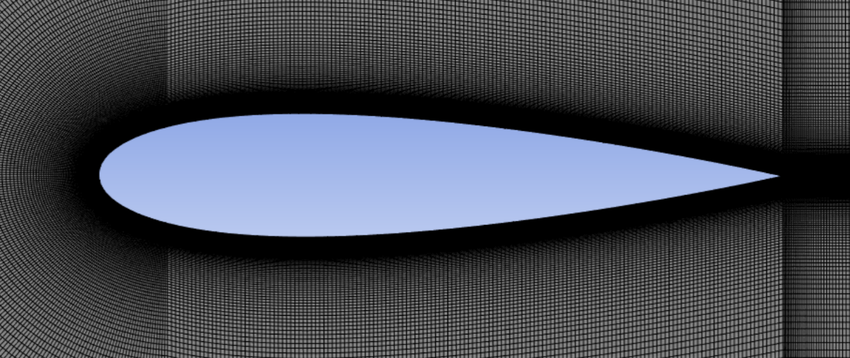
Figure 4: Local detail of airfoil grid

2.2.2. Mesh quality

Mesh quality affects the accuracy of the simulation and the stability of the data. The mesh quality of this study is judged by the following indicators:

i. Mesh skewness

Skewness is one of the main indicators of mesh quality, which determines the degree of closeness of a mesh face or mesh unit to the ideal geometry (i.e., equilateral or equiangular). Skewness of 0 indicates that the unit cell is equilateral (best). The value of 1 indicates that the unit cell is completely deformed, and mesh cells with a skewness greater than 1 are invalid. As shown in Figure 5, most mesh units have a skewness between 0 and 0.2. So, the model has good skewness quality.

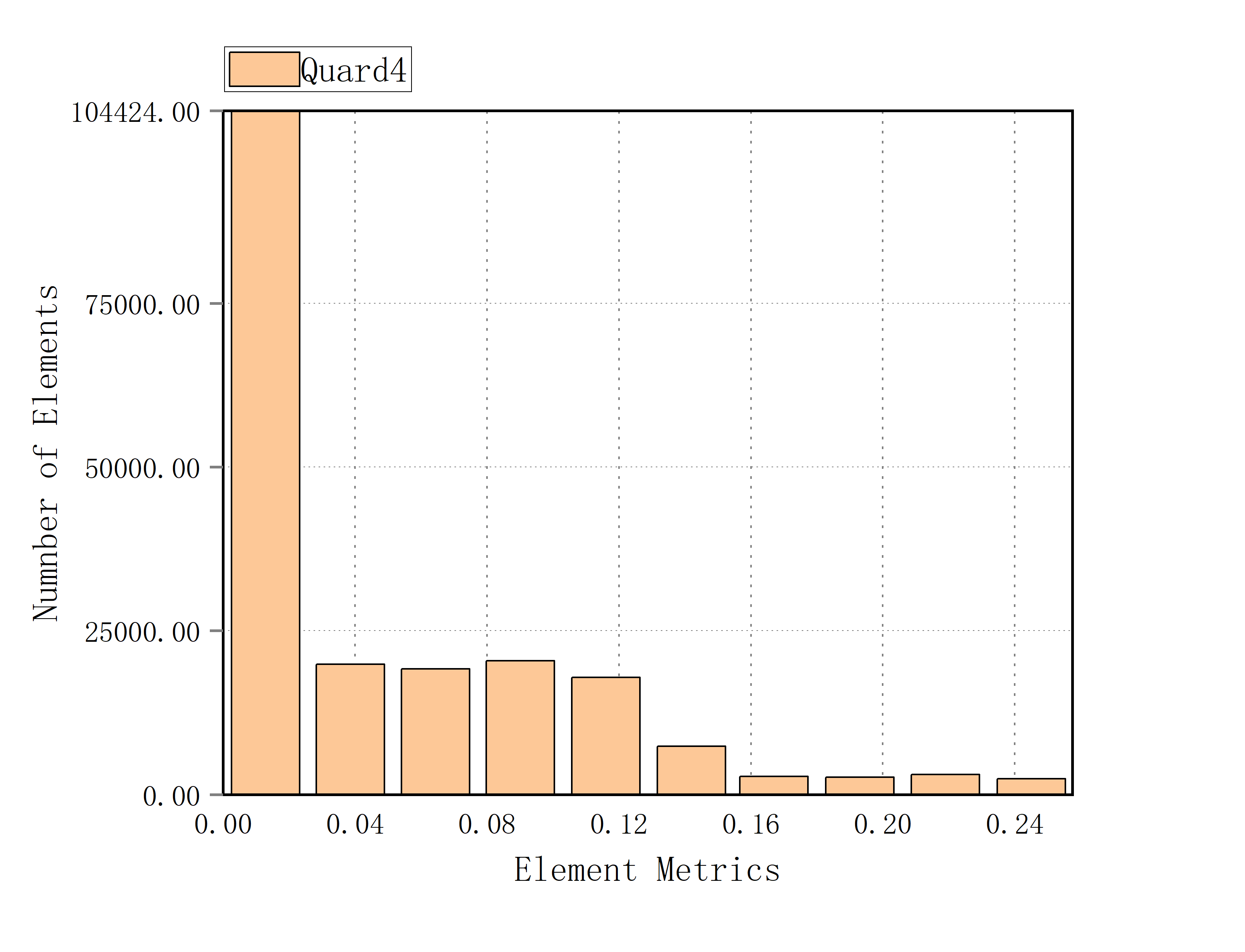
Figure 5: Grid skewness

ii. Orthogonol Quality

Orthogonality is another important indicator of mesh quality. The closer the orthogonal quality value is to 1, the more uniform the mesh unit size and shape, and the numerical solution is usually more stable. As shown in Figure 6, most mesh units have an orthogonal quality between 0.9 and 1, with an average value of 0.992. So the model has good orthogonal quality.

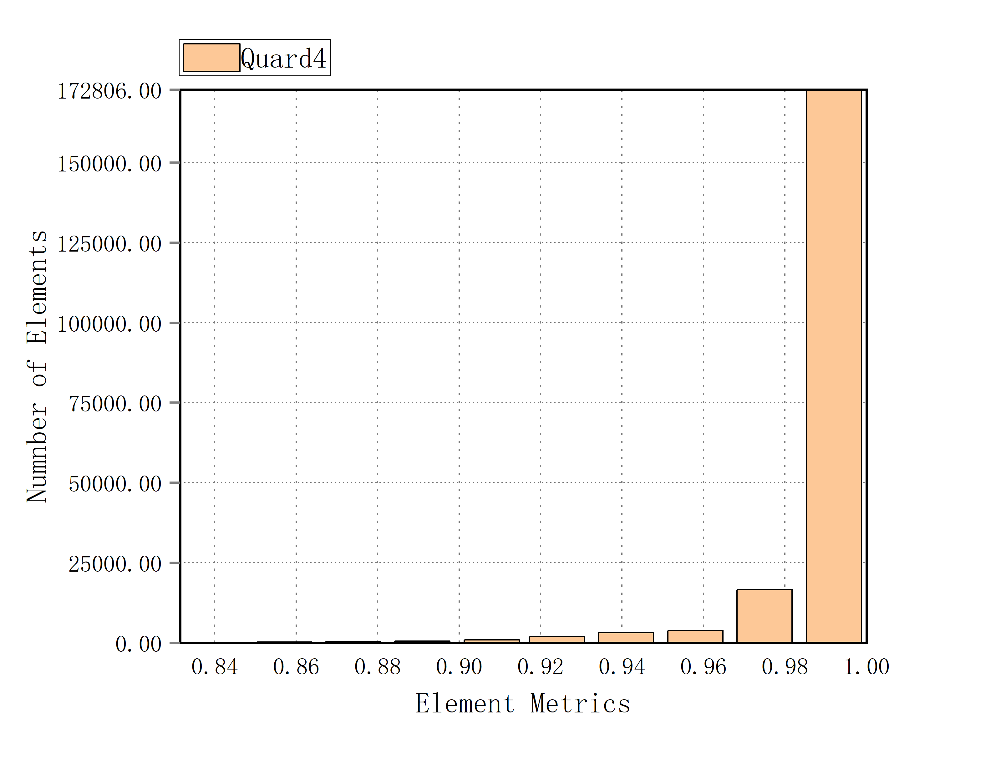
Figure 6: Orthogonal mass

In addition, there are a series of evaluation indicators such as mesh aspect ratio, warp coefficient, and mesh unit quality coefficient to judge the quality of the mesh. The model performs well in other indicators except for the aspect ratio and mesh unit quality coefficient, which are slightly poor. Therefore, the overall mesh quality of the model is relatively high.

2.3. Control equation

Boundary conditions refer to the physical properties or conditions on the surface of the region, representing the specific flow variables of the physical model. To obtain accurate numerical results, this paper sets 1000 iterations and a convergence error of 10^-6 for CFD simulation to ensure the results are converged. Table 1 displays the specific parameters of the boundary conditions used in the model's calculation. The basic control equations used in this paper are the incompressible continuity equation, Navier-Stokes equation, and S-A (Spalart-Allmaras) turbulence model equation.

The expressions of the continuity equation are as follows[13]:

\( \frac{∂ρ}{∂t}+∇\cdot (ρ\vec{V})=0\ \ \ (1) \)

\( \frac{∂}{∂t}(ρ\vec{V})+∇\cdot (ρ\vec{V}\vec{V})=-∇p+∇\cdot (\overline{\overline{r}})+ρ\vec{g}+\vec{F}\ \ \ (2) \)

The expression of the Spalart-Allmaras turbulence model equation is as follows [14]:

\( \frac{∂}{∂t}(ρ\widetilde{ν})+\frac{∂}{∂{x_{i}}}(ρ\widetilde{ν}{u_{i}})={G_{v}}+\frac{1}{{σ_{\widetilde{ν}}}}[\frac{∂}{∂{x_{j}}}\lbrace (μ+ρ\widetilde{ν})\frac{∂\widetilde{ν}}{∂{x_{j}}}\rbrace +{C_{b2}}ρ{(\frac{∂\widetilde{ν}}{∂{x_{j}}})^{2}}]-{Y_{v}}+({S_{\widetilde{ν}}})\ \ \ (3) \)

2.4. Boundary conditions

The simulation parameters and boundary conditions set in this study are as follows:

Table 1: Parameters and boundary conditions

3. Results and discussion

3.1. The variation curves of lift coefficient with angle of attack under variant Reynolds numbers

In this paper, the lift ratio graphs for Reynolds numbers varying between 3×10⁵ and 5×10⁵ as well as angles of attack between 0° and 20° are plotted in Figure 7, compared with experimental data. From Figure 7, it is evident that the lift coefficient increases approximately linearly with the angle of attack when the attack angle is between 0° and 8°. This is mainly because the airflow maintains a relatively stable adhesion state on the airfoil surface. So, the airfoil can effectively generate lift at this angle of attack. Within the range of 8° to 14°, as the angle of attack continues to increase, the attached layer on the airfoil surface gradually thickens, causing the surface flow to separate and form vortices in the wake area, resulting in a slower rise in the lift coefficient. Within the 14° to 16° range, all curves successively reach the stall point, and the lift coefficient rises to the highest value. Subsequently, due to the severe separation of streams across the airfoil’s upper surface, the lift coefficient drops sharply.

The results show that there are slight differences in the lift coefficient curves at variant Reynolds numbers. In the near-linear growth stage of 0° to 8°, the lift coefficients of the airfoil at different Reynolds numbers are approximately equal. However, within the range of 8° to 20°, the lift coefficient rises slightly with the increase of Reynolds number, and the stall angle and the corresponding lift coefficient at variant Reynolds numbers are slightly different. The airfoil has a larger stall angle and a higher corresponding lift coefficient under higher Reynolds number conditions because the flow at higher Reynolds numbers has greater adhesion, leading to delayed flow separation and maintaining a higher level of lift.

To verify the accuracy of the model, the lift coefficient computation findings and the experimental data carried out by Jacobs, Timmer and Robert were compared [15-17]. It demonstrates that the outcomes of the simulation agree with the experiment findings at small angles of attack of 0° to 6°. While the angles of attack are larger, the two are different, but the trends are still relatively consistent.

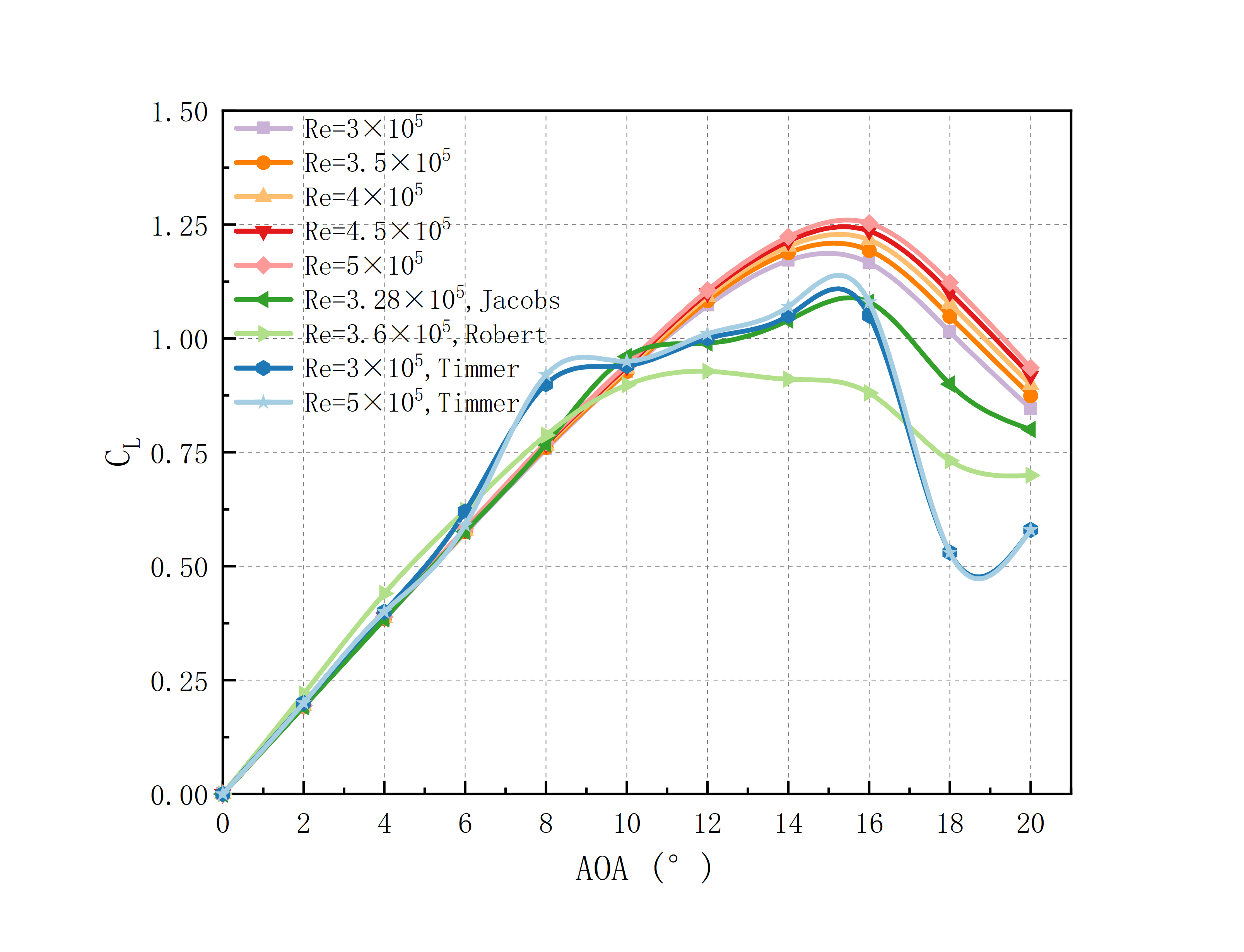
Figure 7: The lift coefficient fluctuation curve with AOA at variant Reynolds numbers

3.2. The variation curves of drag coefficient with angle of attack under variant Reynolds numbers

Since the single lift coefficient cannot fully evaluate the airfoil’s overall performance, the coefficient of drag should also be considered. The curves of drag ratio at Reynolds numbers varying between 3×10⁵ and 5×10⁵ as well as angles of attack between 0° and 20° are depicted in Fig 8, compared with experimental data. Combined with the lift coefficient curve, it can be seen that before the stall, the growth rate of the drag coefficient boosts slowly with the increase of the angle of attack. It is mainly because at smaller angles of attack, the degree of flow separation is low, and the formation and development of vortices are relatively slow. So the flow is more stable. However, after stall, as the degree of flow separation further intensifies and the vortex area further expands, the turbulence level of the flow increases sharply. As a result, the pressure and drag rise rapidly, and the drag coefficient has an accelerated increase.

Similar to the lift coefficient, before stall, the flow adhesion and flow characteristics at variant Reynolds numbers are similar. So, the drag coefficients are approximately equal. After the stall, the drag coefficient of the airfoil at higher Reynolds numbers is slightly smaller than that at lower Reynolds numbers, and the growth rate is relatively slow. This is mainly due to the larger stall angle and stronger flow adhesion at higher Reynolds number conditions, leading to delayed flow separation and reduced drag coefficient and its increase rate.

The simulation results of the drag coefficient are compared with the experimental data. At small angles of attack of 0° to 8°, the simulated outcomes match the experimental findings. While at larger angles of attack, the simulation results are consistent with Timmer at Reynolds number of 5×10⁵, but different from the other three groups of experimental results. In general, the trends are the same.

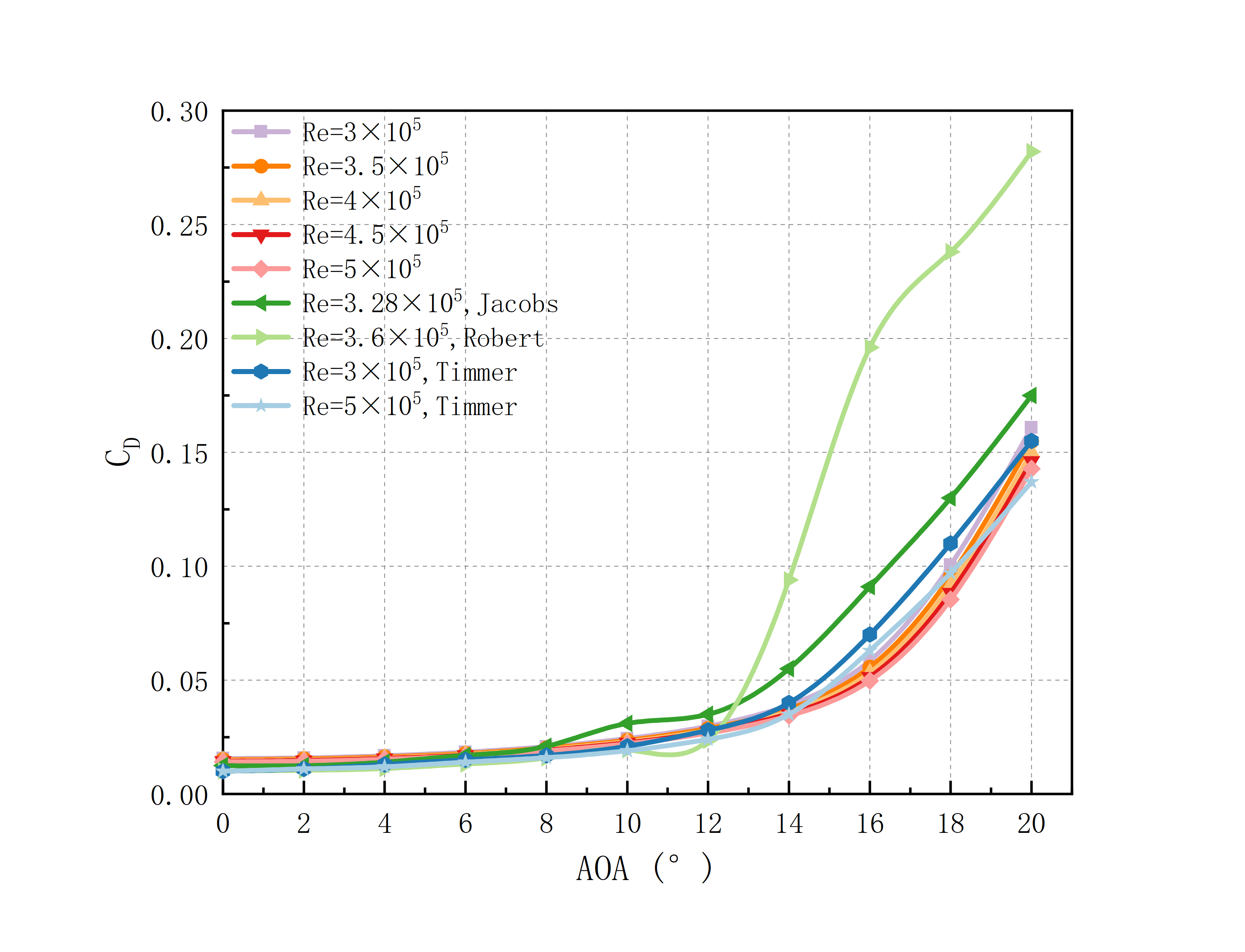
Figure 8: The drag coefficient fluctuation curve with AOA under variant Reynolds numbers

3.3. Pressure contours at variant angles of attack and Reynolds number

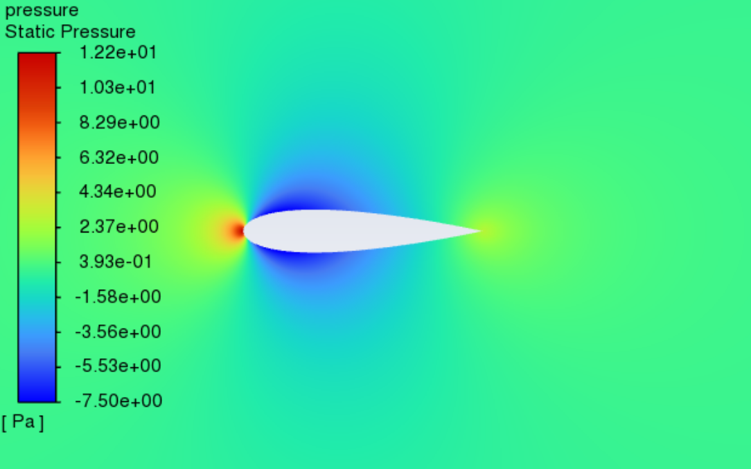
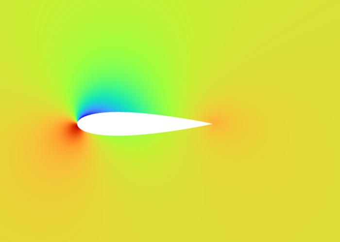
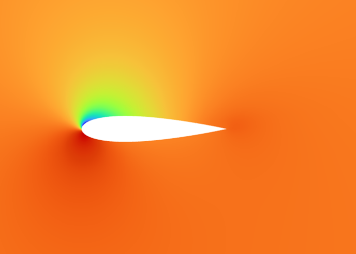
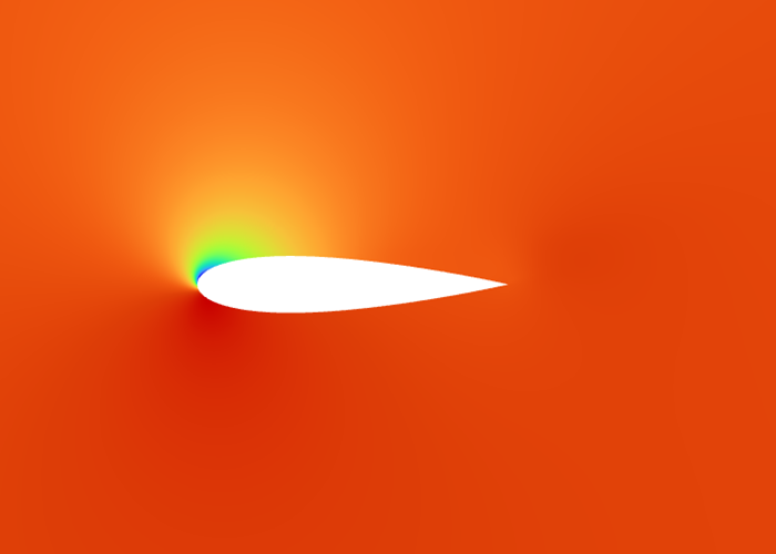
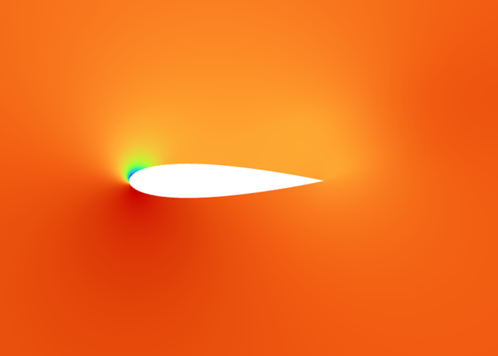
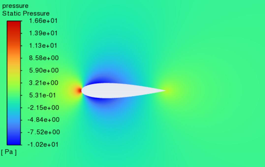
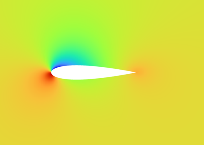
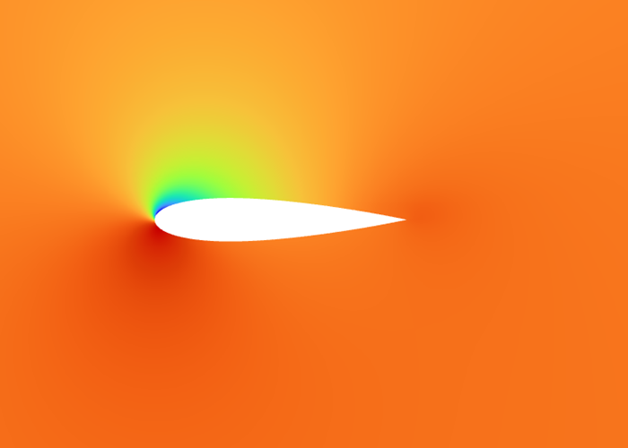
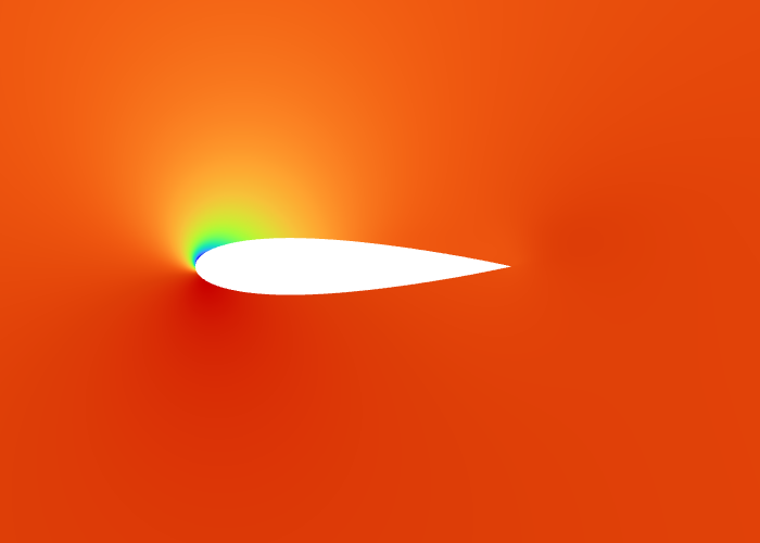
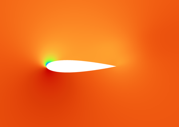
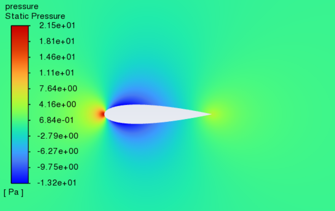
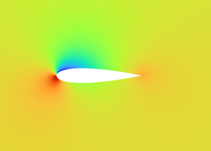
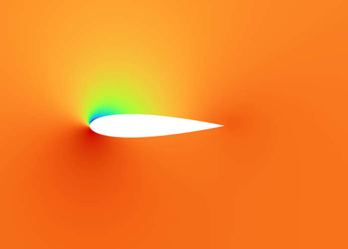
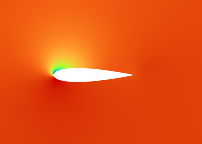
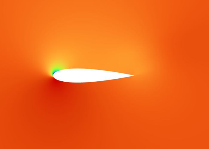
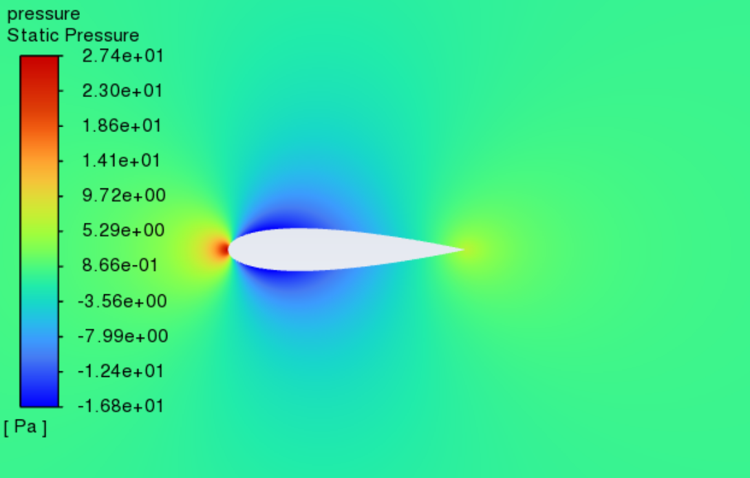
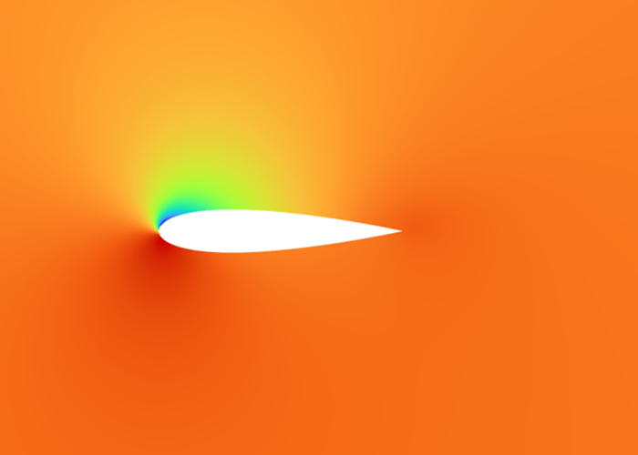
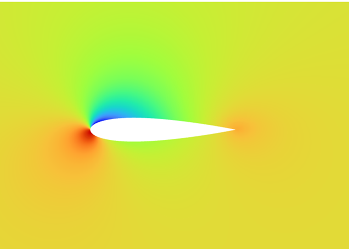
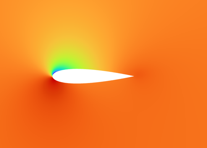
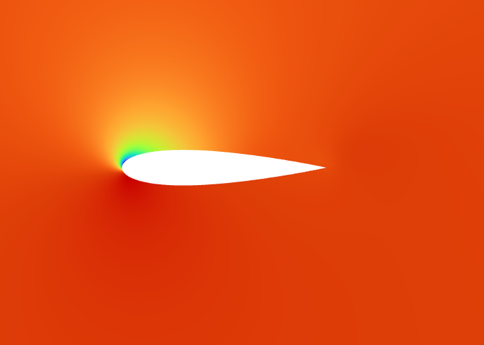
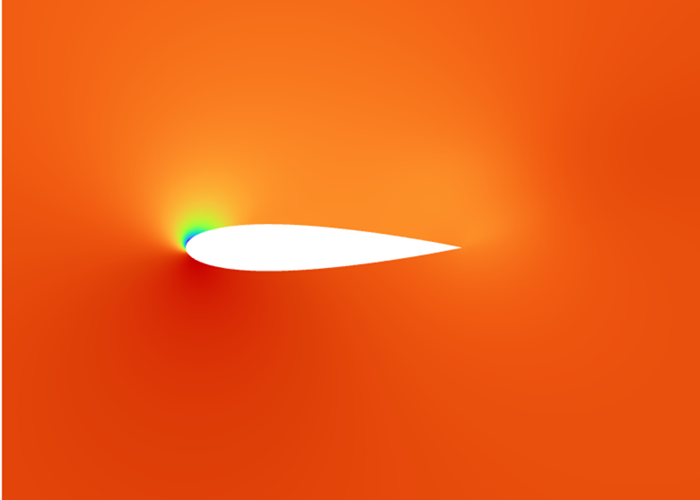
Figure 9 shows the static pressure cloud contours of NACA0018 at Reynolds numbers varying between 3×10⁵ and 5×10⁵ as well as angles of attack between 0° and 20° Within this range, the pressure distribution is unaffected by the Reynolds number. It can be seen from the figure that the stagnation point is located at the leading edge, where the static pressure is the highest. As the angle of attack increases, the pressure centre of the low-pressure area on the upper surface gradually moves towards the leading edge. The static pressure on the airfoil's upper surface gradually decreases, while the pressure on the lower surface is relatively high. According to the lift theory and Bernoulli's principle, the airflow accelerates on the airfoil’s upper surface, causing a decrease in the pressure on the top surface. At the same time, because the pressure on the lower surface is relatively high, the airflow can effectively promote the wing to move upward to generate lift. When the angles of attack are small, as the angle of attack increases, the acceleration of the airflow on the upper surface rises, and the lift rises accordingly. However, when the angles of attack are large, flow separation and stall phenomena begin to occur, leading to a decrease in lift and a sharp increase in drag. Combined with Figures 7 and 8, it can be seen that the change in pressure distribution with the angle of attack is consistent with the change in lift and drag coefficients with the angle of attack.

Re=3×10⁵

Re=3.5×10⁵

Re=4×10⁵

Re=4.5×10⁵

Re=5×10⁵

Figure 9: Pressure contours at variant Reynolds numbers and angles of attack

4. Conclusions

This paper discusses the airfoil NACA 0018’s aerodynamic properties under the Reynolds numbers varying between 3×10⁵ and 5×10⁵ as well as angles of attack between 0° and 20° using ANSYS Fluent. Spalart-Allmaras turbulence model proves to be an appropriate model for these simulations as the results are comparable with the experimental data acquired from reliable sources. The results show that the lift ratio rises first and then drops with the increase of the angle of attack, while the drag ratio rises with the increase of the angle of attack at a faster rate. The change in the pressure distribution is consistent with the changing trend of the lift and drag ratios. The increase of Reynolds number will slightly make the stall angle delay, the lift ratio rise and the drag ratio drop at a large attack angle. However, the Reynolds number essentially does not affect the distribution of pressure. Therefore, NACA 0018 has a higher lift and lower drag when the angle of attack is 12°~14° and the Reynolds number is 5×10⁵. This condition is selected as the best condition of aerodynamic properties.

This study can promote the development of airfoil flow theory at low Reynolds number, the optimization of airfoil design and the practical application at low Reynolds number. However, there are still some limitations in this research, such as the Reynolds number range and the attack angles are not wide, and the difference between the experimental results and the experimental results is comparatively big when the angle of attack is large. Based on the shortcomings and research results, the future research work is further proposed:

First, studying the aerodynamic properties of NACA 0018 under a wider Reynolds number range as well as a larger scope of attack angles. Second, dividing a more detailed computational domain to consider laminar flow and turbulent flow respectively. Third, improving the element quality and aspect ratio of the grid to optimize the simulation results. Finally, selecting a model with a relatively small error for simulation, especially when the angle of attack is large.

Acknowledgements

All the authors contributed equally, and their names were listed in alphabetical order.